Ocean Debris-Detecting Autonomous Underwater Vehicle (AUV)
Overview of Work:
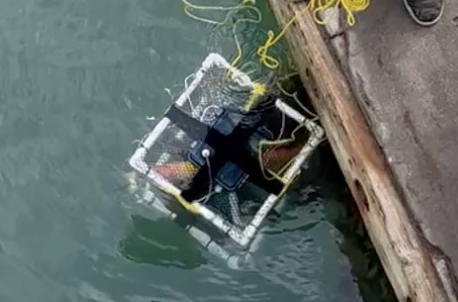
Worked in a team of 4 to design and deploy an AUV utilizing a pressure sensor, thermistor, and magnetometer to map the metal debris distribution on the ocean floor of Dana Point Harbour, and back-calculate debris drop locations using the principles of geostrophic balance.
Key outcomes:
- Built custom operational-amplifier circuits to scale analog sensor outputs to the input range of a Teensy 4.0 to achieve higher resolutions
- Troubleshot circuits and hardware during deployment, conducted tests post-deployment to find and assess key failure modes
- Utilized oscilloscopes, multimeters, and other electronic test instruments to test and debug circuit outputs and I2C communication protocols
- Programmed feedback control loops in C++ for AUV depth and surface control
- Utilized MATLAB to process collected data, perform signal processing algorithms (Fast Fourier Transform), and create 2D and contour plots
Introduction and Background
The goal of this project was to explore the potential of using an autonomous underwater vehicle (AUV) to map seafloor debris and determine their water surface entry point. The United Nations Educational, Scientific, and Cultural Organization estimates there are three million shipwrecks worldwide, among other catastrophe-induced ocean debris. These wreckages are artifacts of human behaviour and are usually investigated to inform historical and cultural accounts. However, these investigations have historically been difficult because current methods to locate wreckages are complex and inefficient. These methods can be improved by detecting magnetic anomalies that indicate metal wreck pieces due to their material composition underwater and reconstructing their points of entry into the water.
An AUV was constructed to collect pressure, temperature, and magnetic flux density data at Dana Point Pier with a sample rate of 10Hz. Pressure and temperature data can be used to create a 3D vector field map of currents in the ocean. The magnetic flux density data can be used to form a contour plot of the magnetic flux density across the ocean floor. These two plots would enable conclusions to be drawn about ferromagnetic materials, which include most metals, on the seafloor and their possible points of entry on the ocean surface through approximating their trajectory along currents while falling downwards.
Initial Setup
Frame and Motor Assembly
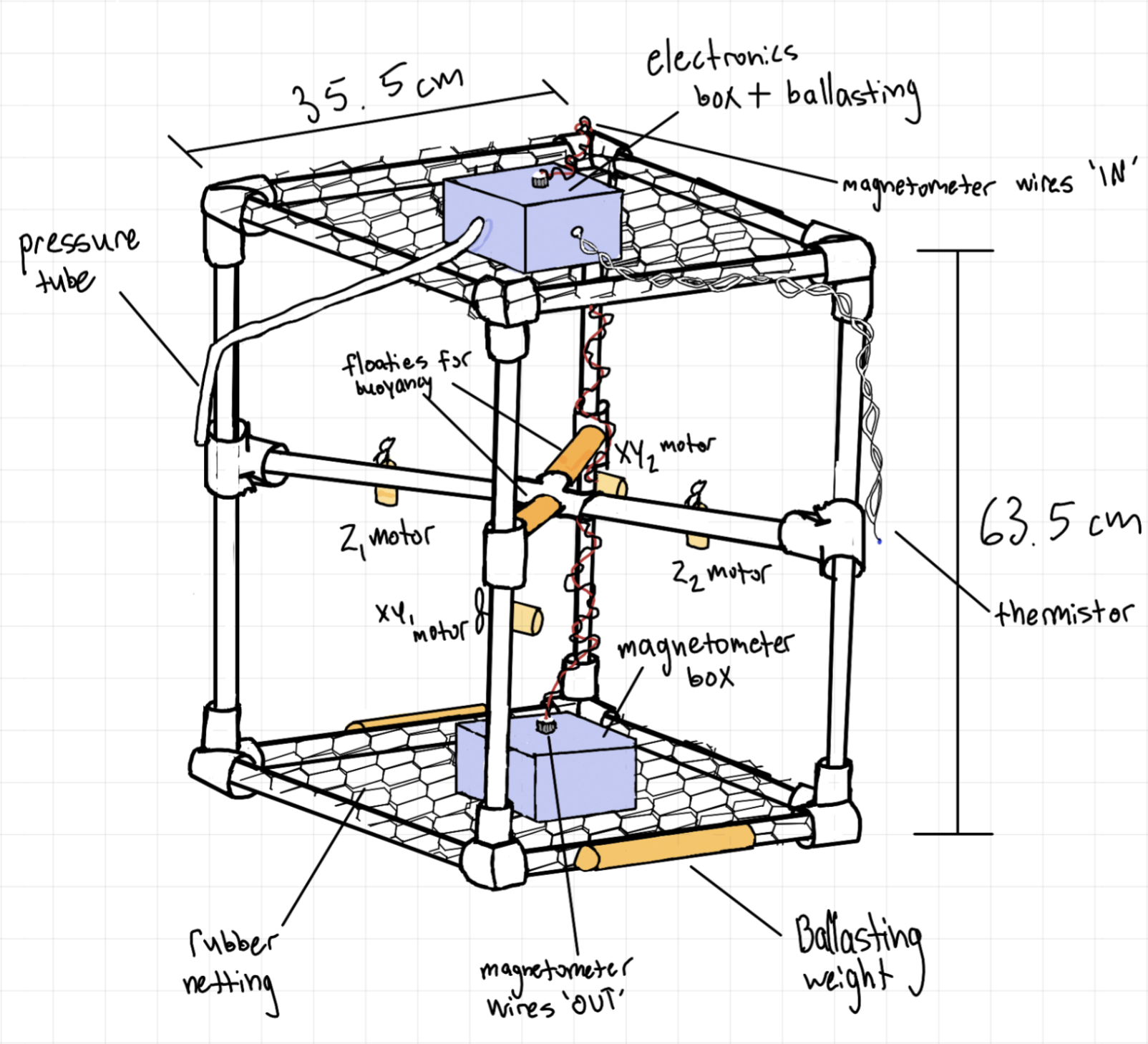
The base AUV model was made out of PVC pipes and pool floaties (to make it neutrally buoyant). 12V DC motors were prepared by fixing a propeller to each shaft, then waterproofed by covering the motor housing with electrical tape and wax, then putting the whole assembly into a film canister.
The motors were tested to pull less than 500mA when supplied with 6V from a DC power supply. They were then mounted to the AUV to give two xy-direction motors and one z-direction motor.
Motherboard Assembly
A battery pigtail, screw terminals, chip sockets, hex buffer, push buttons, slider switches, and female headers were soldered to the AUV PCB, in addition to components that would ensure the safety of the board, such as resistor networks, voltage regulators, motor/battery fault detect LEDs etc. Components such as the IMU and SD card slot came presoldered. The back of the motherboard was covered with an insulating foam sheet to prevent short circuits.
Validation, Calibration, and Error Measurement
The motherboard was validated by running a simple Arduino sketch on the Teensy 4.0 to blink several LEDs (confirming overall board power, IMU power, Teensy 4.0 power, and SD card connection), and turn on a motor for four seconds. The SD card was verified to be saving INF and BIN files when the sketch ran, and when opened in MATLAB, acceleration, magnetic field strength, roll, pitch, and yaw values (calculated from the IMU), and motor PWM values were confirmed to be saved.
Another Arduino sketch was run to confirm all the motors could be driven.
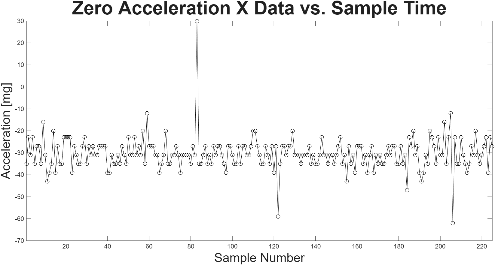
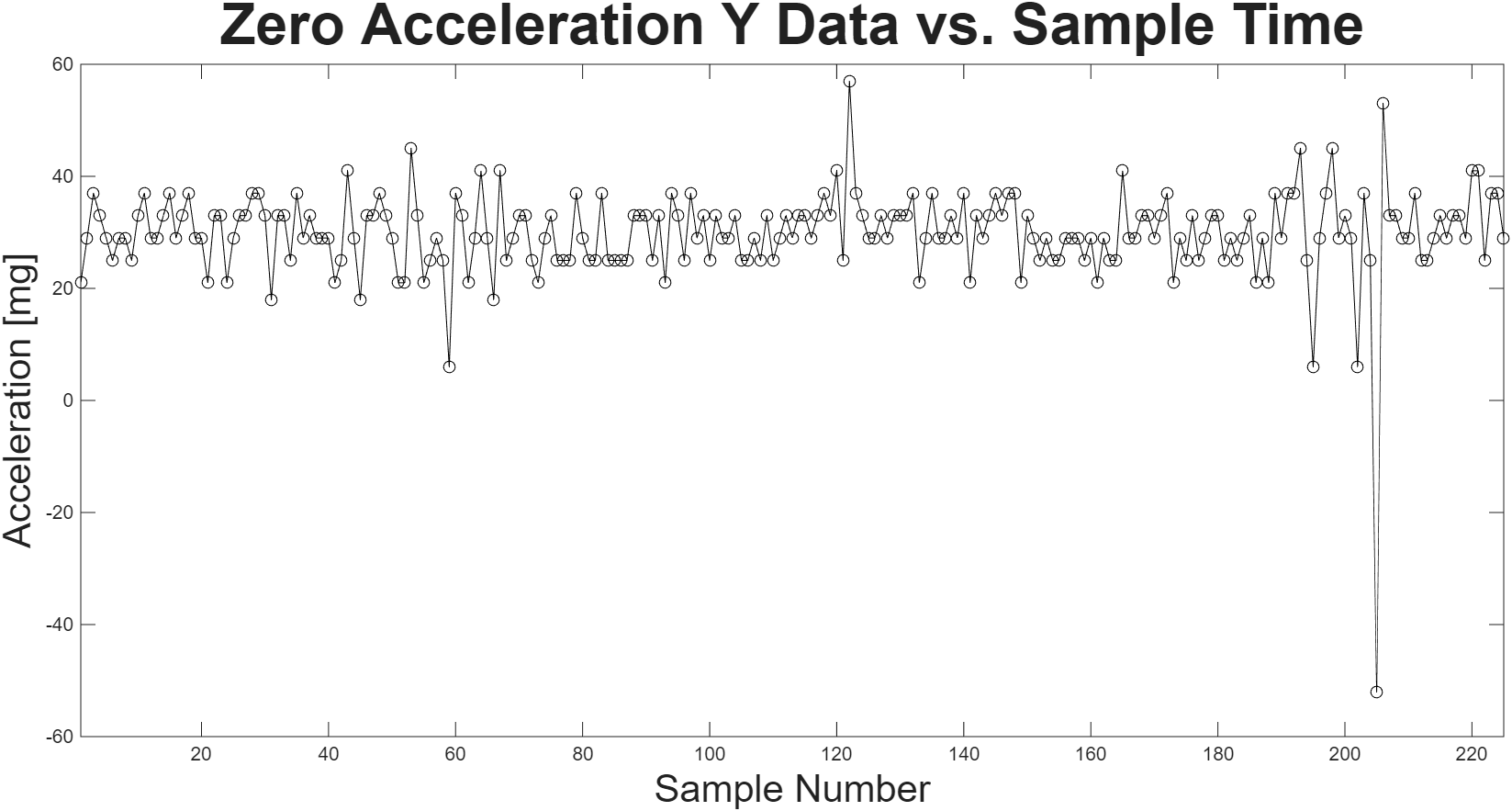
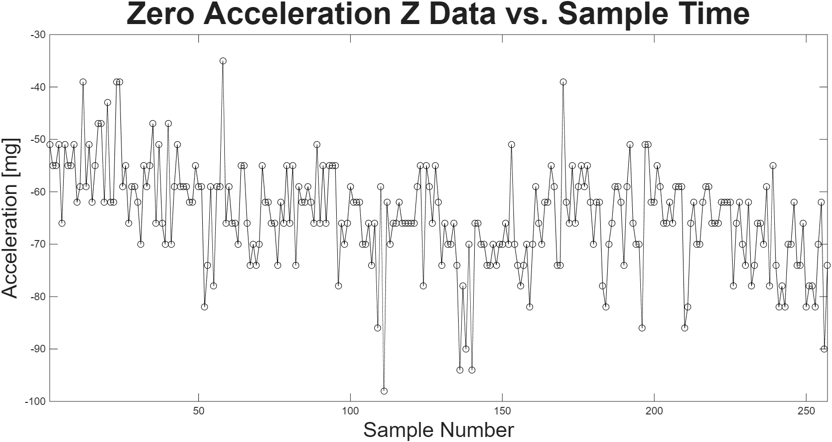
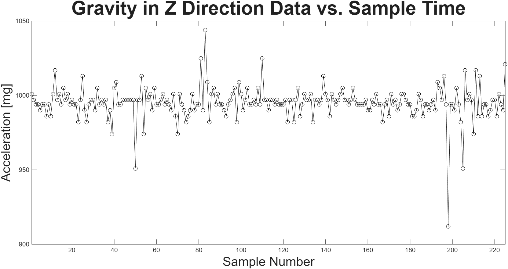
The saved accelerator data was analyzed when the board was static. The data needed to be converted from the saved units to \(ms^{-2}\). This was done by comparing the value read when the sensor experienced acceleration due to gravity (ie. when one axis of the sensor aligned with the global z-axis) to the value read when the sensor experienced 0 acceleration. The equation for this was \(\text{accelerometer unit}=\frac{9.81}{\text{value for accel due to gravity - value for zero}}ms^{-2}.\) The value for acceleration due to gravity in the z direction read 995.2089 accelerometer units. The value for zero in the z direction read –64.6498 accelerometer units. Using the equation, one accelerometer unit is 0.0093 \(ms^{-2}\). All acceleration readings from the Teensy could be converted to \(ms^{-2}\) by multiplying them by this value. The following figures show the zero acceleration data versus sample time for all three axes, and the acceleration due to gravity data for the z-axis. The mean, standard deviation, estimated standard error, and 95% confidence interval were found using a MATLAB script.
Open-Loop Control Navigation
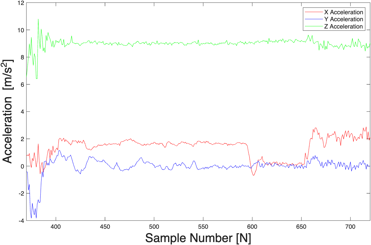
C++ code was written so the AUV could traverse through an obstacle course. After the obstacle course deployment, the on-board accelerometer readings were plotted, as shown in Figure X.
The governing equation for the AUV’s acceleration is \(mx"=mg+F_{thrust}-F_{buoyancy}-bx'\). The AUV was neutrally buoyant, so \(mg\) and \(F_{buoyancy}\) cancel. \(b\) represents the damping constant, so when \(x'=0\), there is no effect of damping (in this case, drag force - resistance from moving through the water) on the robot. Acceleration will be highest when there is no damping, so we remove the \(bx'\) term. So the peak acceleration from rest is \(x"_{peak}=\frac{F_{thrust}}{m}\).
Using the x-direction for calculations (because it would have less interference compared to the x-direction and y-direction, since the AUV started from rest and there was significant tilt by the time the x-direction and y-direction acceleration was being affected), the theoretical thrust force could be calculated using a thrust vs duty cycle equation. For the motors used, \(F_{thrust}=|-0.6871\text{Duty Cycle}+0.0593|\). The duty cycle could be calculated using \(\text{Duty Cycle}=\frac{|\text{PWM}|}{255}\) since 255 is the maximum PWM the motors can run at. The code used had the PWM set to -100 for downward motion in a single motor, giving a duty cycle of 0.3922. This gives a theoretical thrust force of 0.2102 N for one motor. The theoretical peak acceleration was calculated using the governing equation. The total mass of the AUV was measured to be 3297.6g = 3.2976kg, giving a theoretical peak acceleration as 0.0637m/s^2. From Figure X, the measured peak acceleration was \(-2.6505ms^{-2}\) in the z-direction. The theoretical value was different from the measured value because the thrust vs duty cycle equation was procured a motor the team did not use, meaning the curve would likely give an inaccurate estimate. Even though we tried to place the robot level in the taken, the robot tilted when the motor started driving, and the motherboard was not level in the box, so the measured acceleration values would contribute to each other’s axes. There was also a lot of noise from the accelerometer and other teams sloshing the water in the tank, which could make the measured acceleration of our robot a lot greater than actually contributed by the motors.
The AUV was programmed to move downward, forward, then upward. The initial large downwards peak in the z-direction represents the z-direction motor activating, moving the AUV downwards. Here, there are fluctuations in the x and y-direction generated from the AUV spinning in the x-y plane when it descended. There is then an upwards peak past the base value in the z-direction caused by the motor deactivating because the AUV was slightly buoyant, making it rise. From around sample number 400 to 600, the forward motors activated, but the AUV made a curve around the obstacle course, causing an increase in acceleration in the x and y-directions. The AUV tilting in various directions while moving also contributed to this increase. Because of buoyancy, the AUV continued rising at the same rate even though the upwards motors was off, so the acceleration hovered at a constant value from around sample number 400 to 650. From around sample number 600 to 650, the AUV reached the surface of the water and stopped tilting, so the x and y-direction data starts to fluctuate around the base value. The z-direction motor activated at around sample number 650, causing the AUV to bob and jitter near the surface of the water, causing reading fluctuations in all three directions. The y-direction reading increased because it started moving in that direction from waves generated from other teams. From this, it is clear thaat open-loop control is not ideal for an autonomous system. Motor behaviour, buoyancy, and waves in the tank threw the AUV off course and resulted in behaviour contrasting its programming.
Sensor Development
The team developed several sensor circuits while determining the project scope. We ultimately decided on using the thermistor, pressure sensor, and a magnetometer to achieve our goals. However, this section outlines all sensor circuits prototyped.
Turbidity Meter
Getting Familiar with Operational Amplifiers
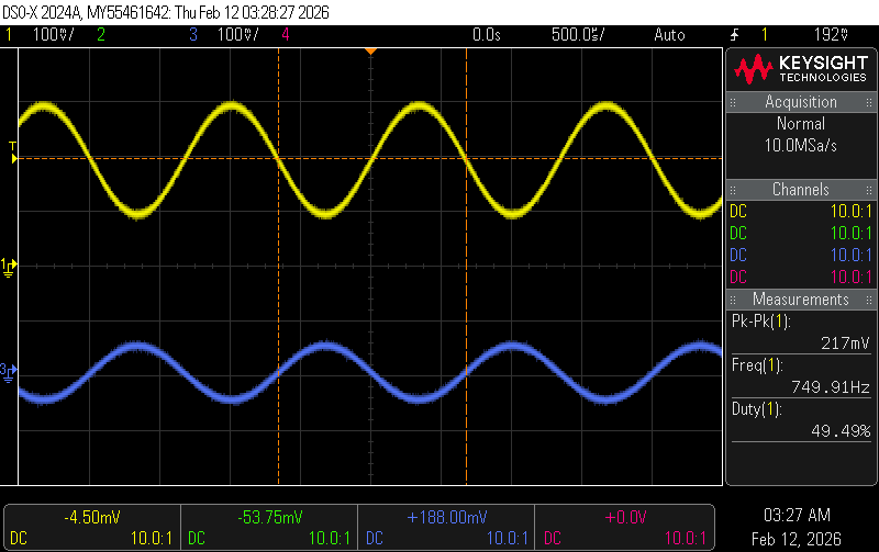
I had no prior experience with operational amplifiers, so to get familiar with them (as they would be needed to scale the sensor outputs to get a better resolution when read by the Teensy 4.0 ADC), I first built a single rail, non-inverting amplifier with a gain of 2. I applied a 100mV amplitude sine wave with a 1V offset, then with an offset of 0V, catching each input and output on an oscilloscope.
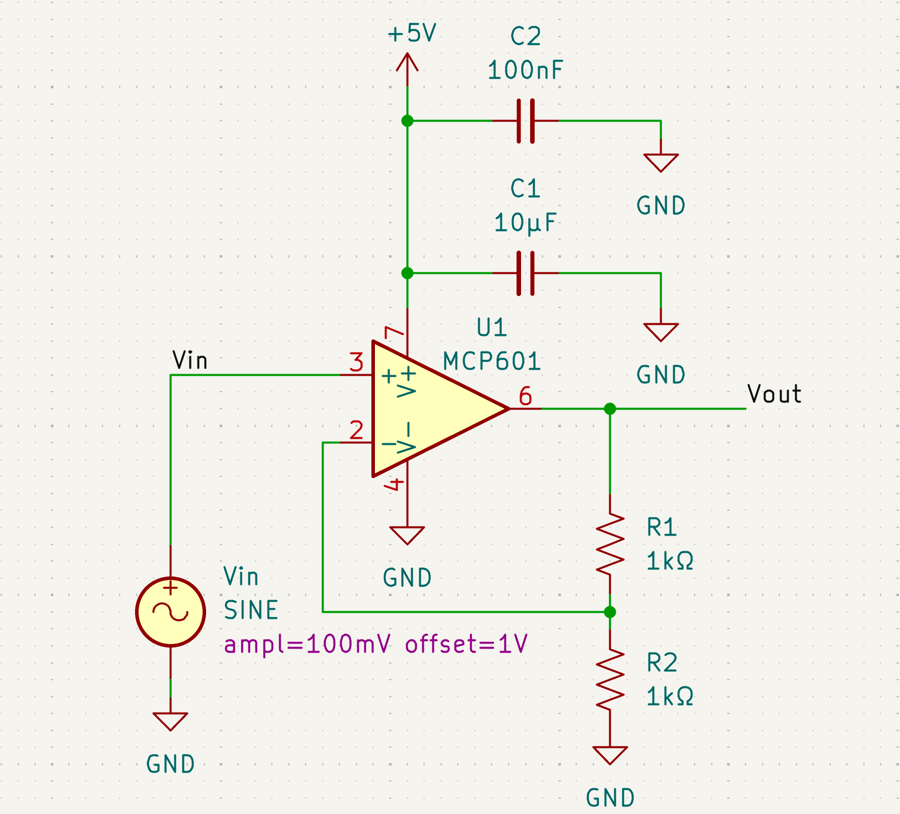
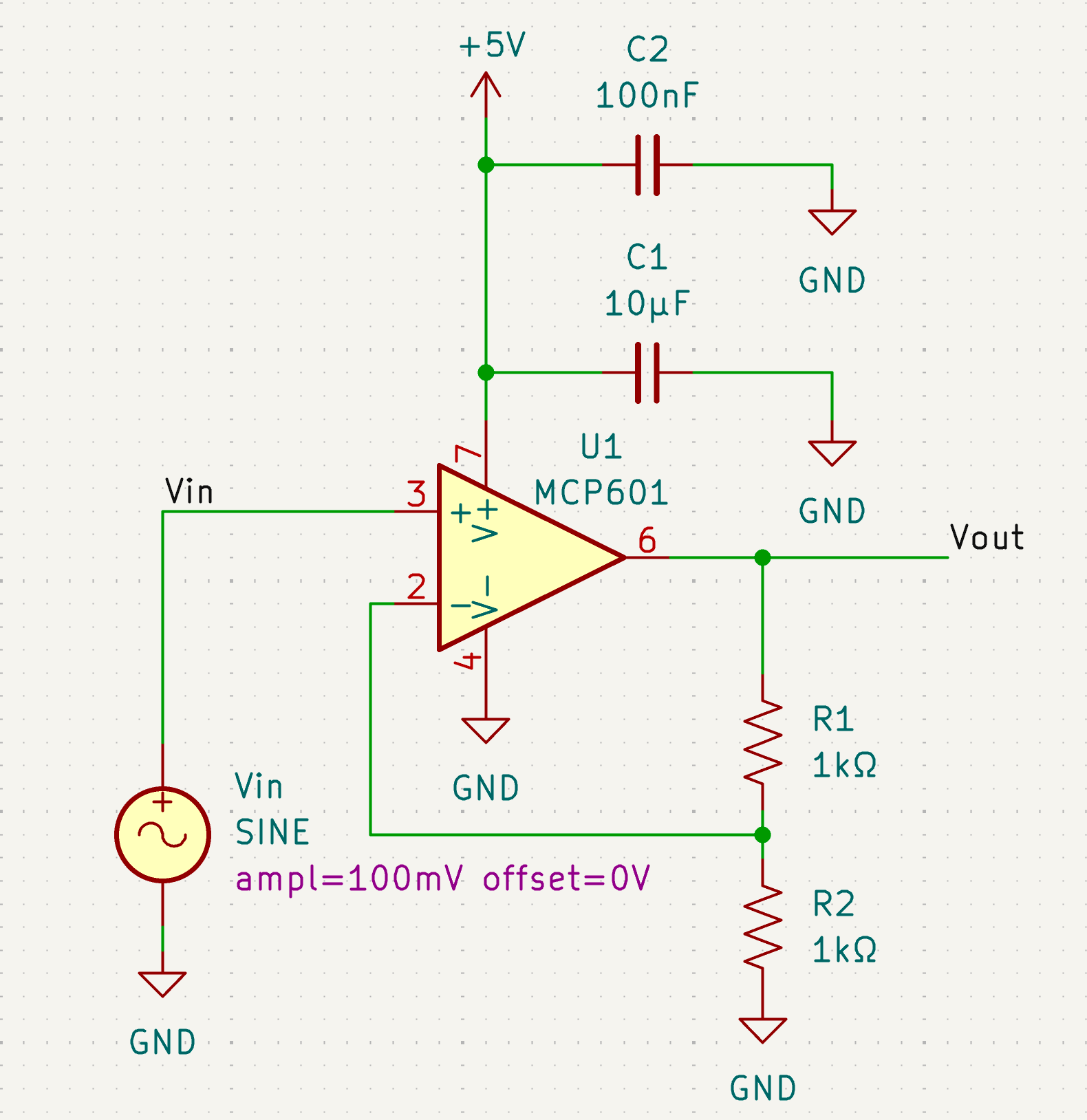
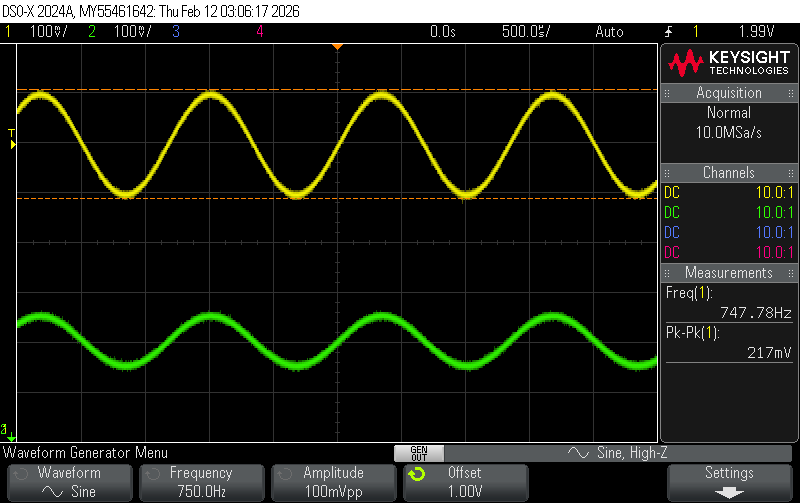
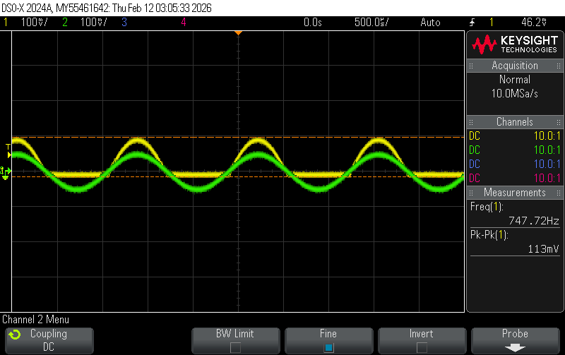
In both traces, the desired gain of 2 was achieved, as seen by the input voltage being scaled by 2 in the output voltage (100mV to around 200mV in the 1V offset one, 100mV to 100mV in the 0V offset one due to clipping). When the signal was sent into the op-amp with a 0V offset, only the positive voltages of the original sine wave show up on the output, with the negative voltages being output as 0V.
The output signal in the 0V offset trace does not obey the equation that describes non-inverting amplifier outputs because I used a MCP601 which is a single supply op-amp, which means it only has +V and GND, so Vout can only be positive. Since the input has a 0V offset, half of the input signal is out of the range of the op-amp (it goes below the minimum possible output), making it look like the op-amp is producing a constant output instead of the ideal sine wave. I learned that this was how op-amps could be used to scale signals, but that I would need to be careful of “railing out”.
Next, I build an offset amplifier that could take the same 100mV amplitude sine wave with a 0V offset and output the full signal. I did this by using a gaim of -2 and a 200mV offset.
Assuming an ideal op-amp (infinitely large input impedance, and \(V_+=V_-\) in negative feedback), \(V_{out} = (1+\frac{R_f}{R_n1})V_+-\frac{R_f}{R_n1}V_in\) where the gain factor is \(-\frac{R_f}{R_n1}\) and the offset factor is \(1+\frac{R_f}{R_n1}\).
If the gain factor is -2, then \(-\frac{R_f}{R_n1}=-2\), so \(R_f=2R_{n1}\). I used \(R_f=20k\Omega\) and \(R_{n1}=10k\Omega\) based on resistor availability.
Since the minimum input voltage would be -100mV, and at this point we want an output voltage of 0V, I substituted these values in to solve for \(V_+\).
\[ \begin{aligned} V_{out}&=(1+2)V_+2V_{in}\\ 0&=3V_-0.2\\ V_+&=0.67 (rounded up so V_{out} doesn't rail)\\ \end{aligned} \]
Using \(\frac{R_g}{R_{p1}+R_g}V_{p1}=V_+\), where \(V_{p1}=5V\) supplied from the 5V power supply into the op-amp to reduce the need for multiple power sources,
\[ \begin{aligned} \frac{R_g}{R_{p1}+R_g}5&=0.067\\ R_g&=\frac{0.067}{5}R_{p1}+\frac{0.067}{5}R_g\\ 74R_g&=R_{p1}\\ \end{aligned} \]
I used \(R_g=2k\Omega\) and \(R_{p1}=148k\Omega\) based on resistor availability. The schematic is shown in Figure x.
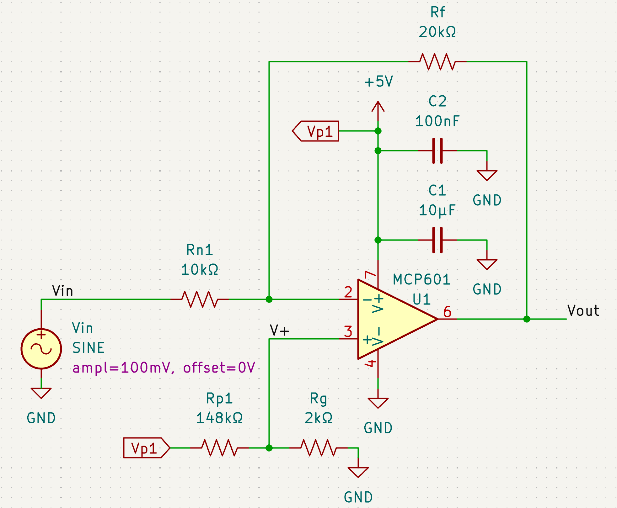
From the oscilloscope trace, compared to the input signal, the output signal has a -2 gain and 200mV offset, which matches the theoretical design.
This design did not have the non-idealities that the non-inverting amplifier has because it included a 200mV offset with -2 gain, so the -100mV input peak can be output as 0V. Since the op-amp is single-rail and cannot handle negative voltages, this prevents the op-amp from resorting to failure mode as seen in the non-inverting amplifier, and the full output sine wave was visible.
555 Timer LED Driver and Transimpedance Amplifier Circuits
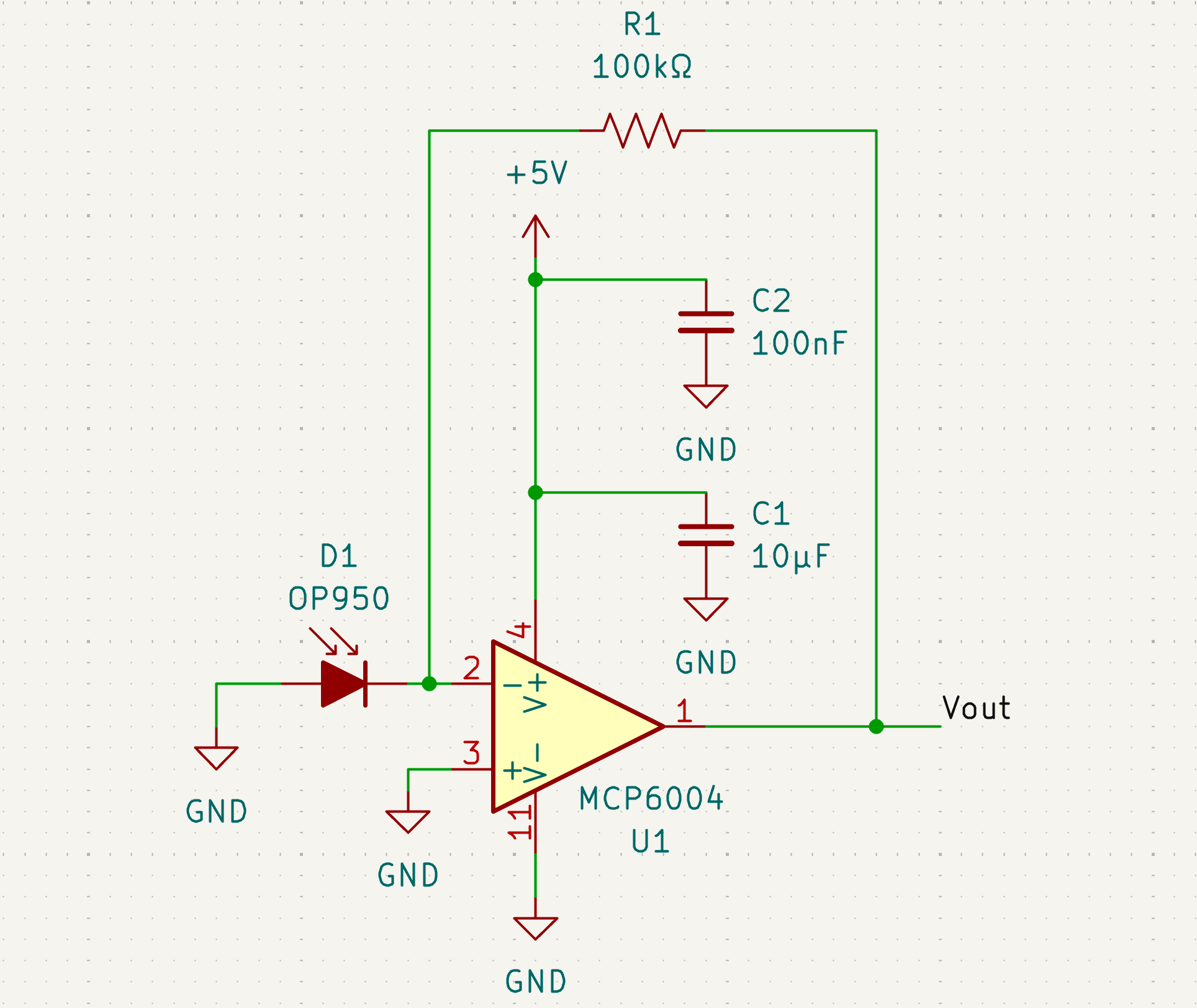
Turbidity meters depend on illuminating a water sample and measuring the ratio of light that passes directly through the sample to light that is scattered 90°. We used an IR LED to illuminate the samples and an IR photodiode to measure the transmitted and scattered light. The photodiode was connected to a transimpedance amplifier circuit to convert the diode current into an output voltage. Figure x shows the schematic of the transimpedance amplifier. Note that since the MCP6004 op-amp contains four op-amps, the unused op-amps were connected as unity gain buffers with inputs and outputs grounded to prevent noise from floating inputs.
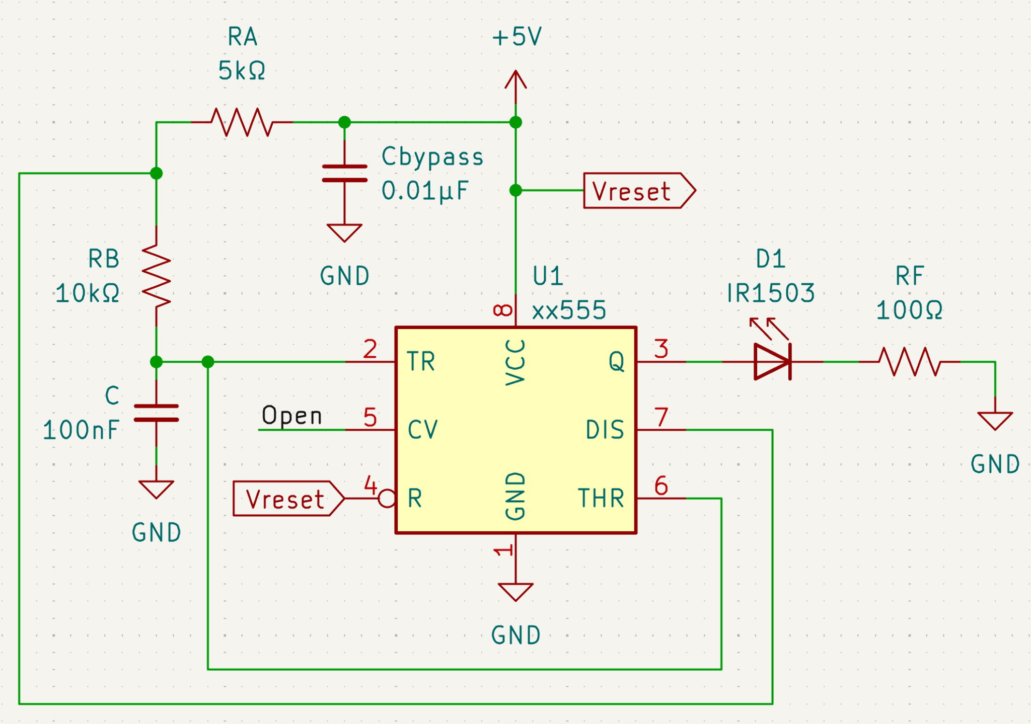
A 555 timer was used to drive the IR LEDs. This was done instead of permanently turning the LEDs high because any ambient light in the water sample would produce an offset voltage in the transimpedance amplifier output. The switching LED would produce oscillatory behaviour so we could measure the peak-to-peak output voltage and thus isolate the voltage caused by the LEDs from ambient light.
We wanted a 500Hz-1kHz square wave with an output waveform duty cycle of about 60% to ensure the LEDs fully illuminated the water sample. From the SE555 datasheet, the output waveform duty cycle was \(\frac{R_A+R_B}{R_A+2R_B}\). This was equated to solve for \(R_A\) and \(R_B\).
\[ \begin{aligned} \frac{R_A+R_B}{R_A+2R_B}&=0.6\\ R_A+R_B&=0.6R_A+1.2R_B\\ 0.4R_A&=0.2R_B\\ R_A&=0.5R_B \end{aligned} \]
So the ratio of \(R_A\) to \(R_B\) is 1:2. Based on the available resistors, and to use an available and suitable capacitor (as shown below), we chose \(R_A=5k\Omega\) and \(R_B=10k\Omega\).
The datasheet also stated the operating frequency was given by \(\frac{1.44}{(R_A+2R_B)C}\). This was equated to 500Hz and 1kHz to solve for the minimum and maximum values of the capacitor.
\[ \begin{aligned} f&=\frac{1.44}{(R_A+2R_B)C}\\ f&=\frac{1.44}{(5000+20000)C}\\ f&=\frac{1.44}{25000C}\\ \end{aligned} \]
\(500=\frac{1.44}{25000C}\) gives \(C_{max} = 115nF\)
\(1000=\frac{1.44}{25000C}\) gives \(C_{min} = 57.6nF\)
Based on the available capacitors, we chose \(C=100nF\) to produce a frequency of 576Hz.
From the IR1503 datasheet, it has a 1.2V forward voltage drop when driving a 20mA current. Since the 555 timer input voltage is 5V, the voltage drop across the current limiting resistor between the LED and ground would be \(5V-1.2V=3.8V\). Using Ohm’s law, an appropriate resistor value was calculated to produce a 20-40mA current through the LED.
\[ \begin{aligned} V_{cc}-V_F&=I_FR_{Fmax}\\ 3.8V&=0.02A*R_{Fmax}\\ R_{Fmax}&=190\Omega \end{aligned} \]
\[ \begin{aligned} V_{cc}-V_F&=I_FR_{Fmin}\\ 3.8V&=0.04A*R_{Fmin}\\ R_{Fmin}&=95\Omega \end{aligned} \]
Based on these calculations we chose 100Ω as the current limiting resistor. Figure x shows the 555 timer schematic.
Circuit Testing and Calibration
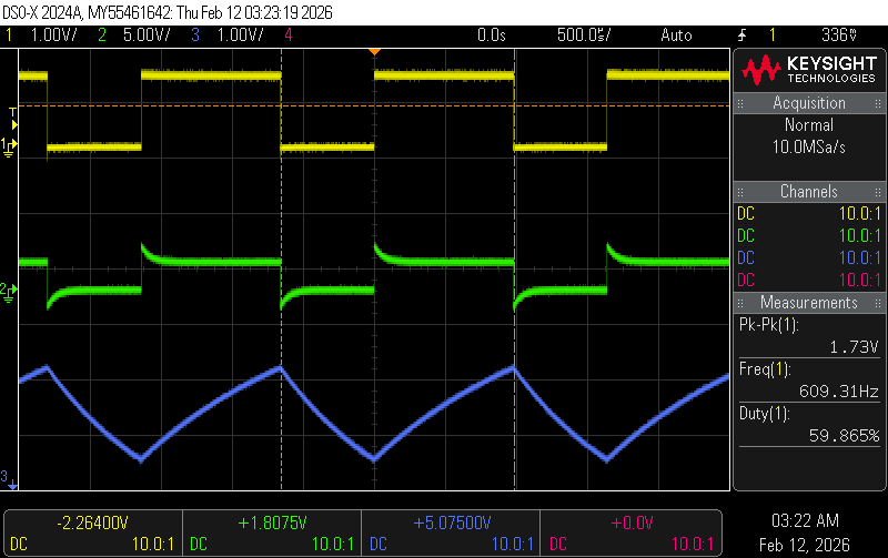
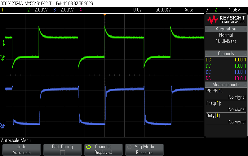
To test the circuits were functioning, we first captured an oscilloscope trace of the 555 timer output to ensure the frequency and duty cycle were correct. In Figure x, the three traces show the 555 timer output, the 555 capacitor node, and the voltage in the middle of the diode resistor string.
We then captured an oscilloscope trace of the transimpedance amplifier output when the photodiode was illuminated by the switching IR LED to ensure the circuit could be correctly driven (shown in Figure x).
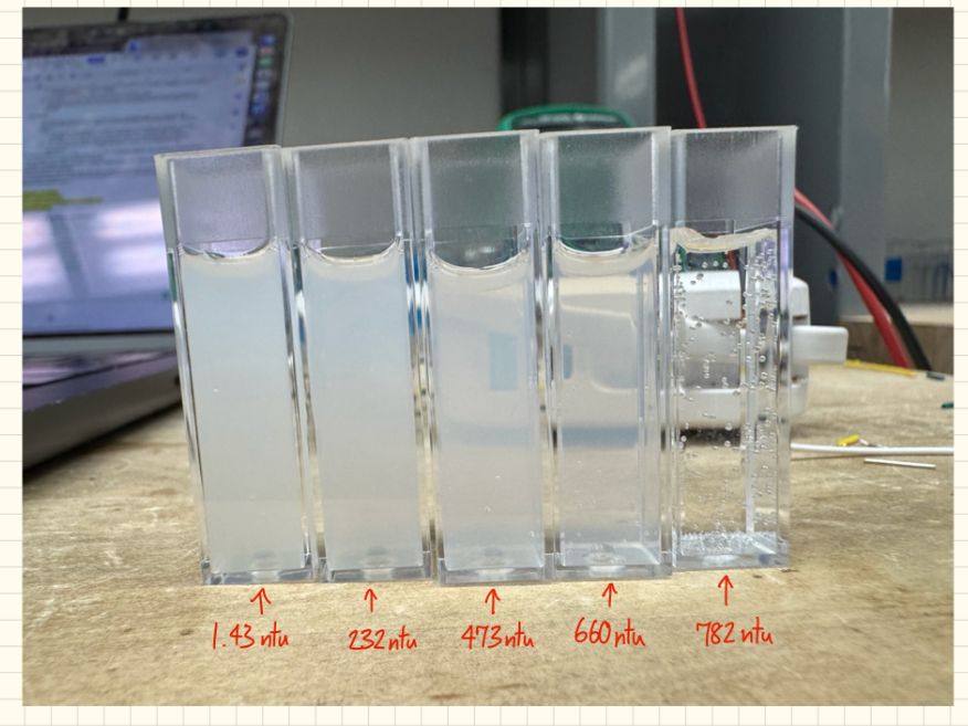
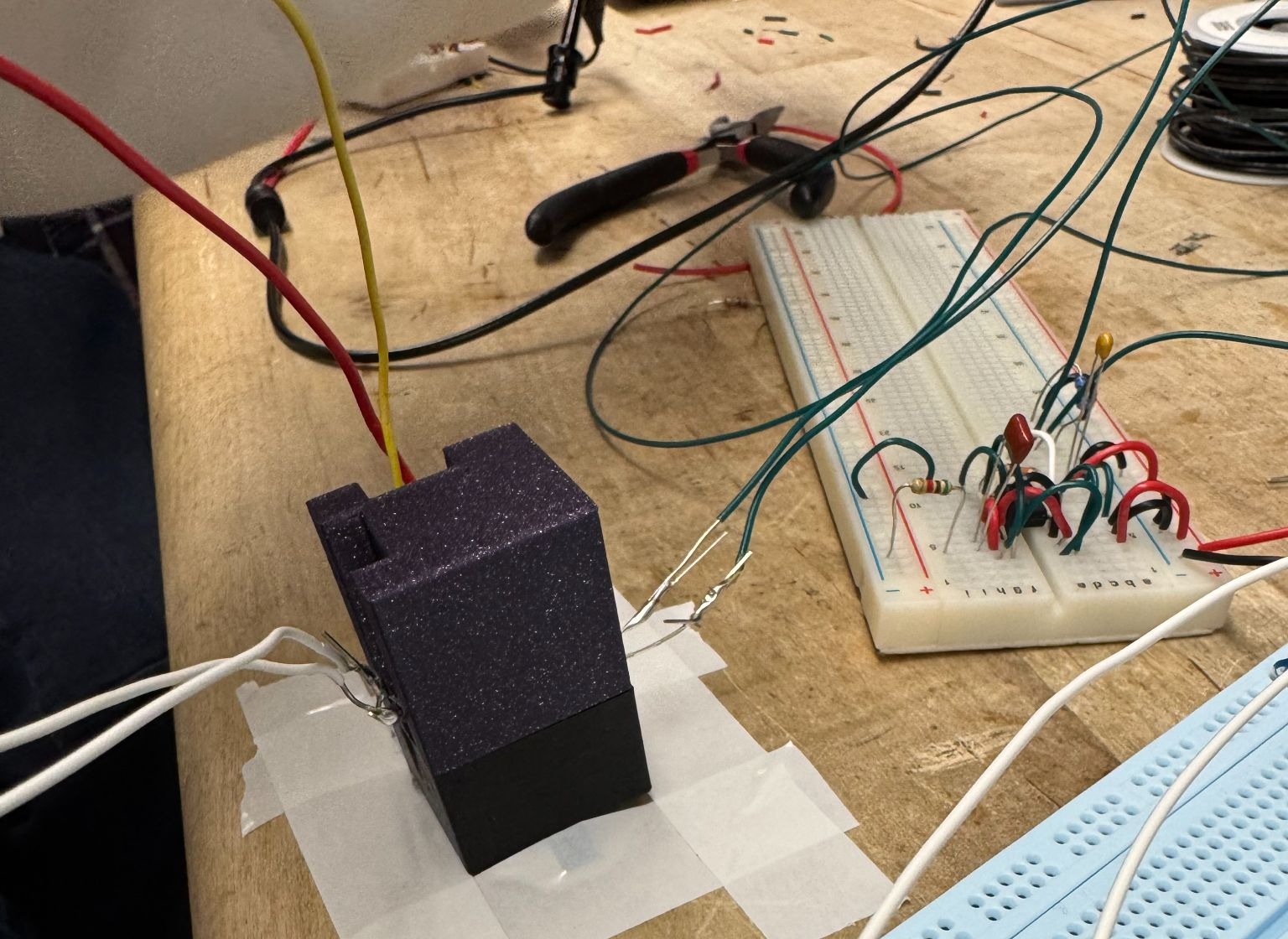
To finalize the turbidity meter, 5 solutions of various turbidities were prepared using milk and water, and checked using the TU-2016 turbidity meter. The solution cuvettes were then placed in a 3D-printed fixture that held one IR LED and two photodiodes in the correct orientation.
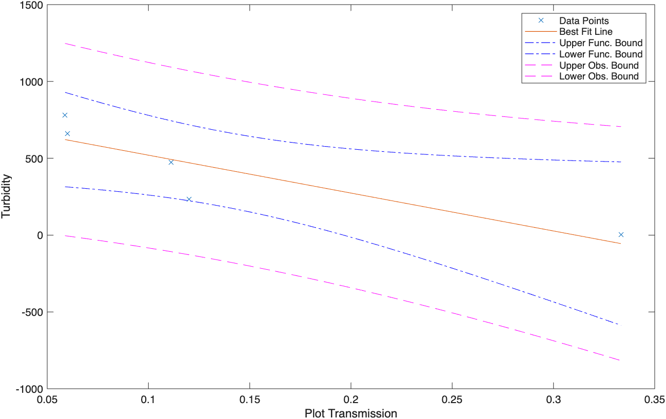
The peak-to-peak voltage of the 90° and 0° transimpedance amplifier outputs were recorded for each solution. The ratio of these voltages were plotted against the calibrated turbidity data to get a calibration curve. The results were plotted in MATLAB and are shown in Figure x.
Depth Sensor
The depth sensing circuit utilized a MPX5700 pressure sensor. This was chosen because of its large operating absolute pressure range (15-700kPa), linear relationship between output voltage and pressure, and easy integration with the AUV.
The estimated deployment depths were 0-40cm. This is much smaller than the operating range of the sensor, so the sensor outputs were shifted and scaled to maximize the resolution of the Teensy 4.0 readings.
From the MPX5700 datasheet, the pressure sensor gives an output voltage of \(V_p=V_s(0.0012858P+0.04)\), with \(V_s=5V\) and \(P\) in kPa. At 0m (sea level), the measured pressure was 96.86kPa. The density of water (ρ) is \(1000kgm^{-3}\), and gravitational acceleration (g) is \(9.81ms^{-2}\). Substituting these values into the equation gives \(P = P_0+\rho gh=96.86+\frac{9810h}{1000}\) relating differential pressure in kPa to depth in meters.
Substituting this and the minimum and maximum depths into the pressure sensor output voltage equation produces a target voltage range of 0.82271294-0.847940336V. This was shifted and scaled to a range of 1.1-2.2V using an offset amplifier with a gain of 43 and a ratio of \(R_g\) to \(R_{p1}\) of 1:4.856. Figure x. shows the schematic of the depth sensor circuit.
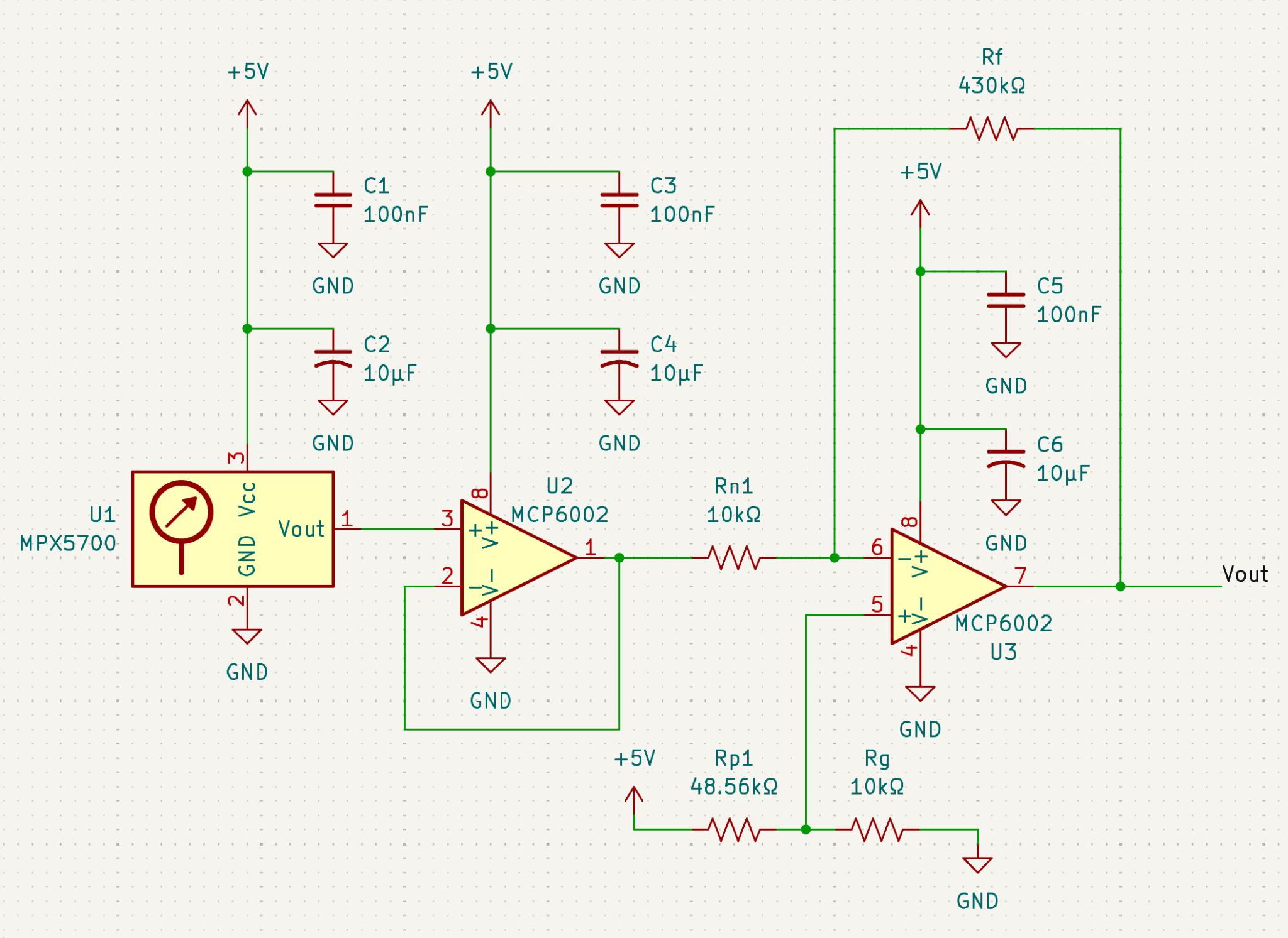
By connecting a tube to the pressure sensor and submerging its other end in a graduated cylinder, the team was able to make a calibration curve of the circuit output voltage to depth. The results were plotted in MATLAB and are shown in Figure x.
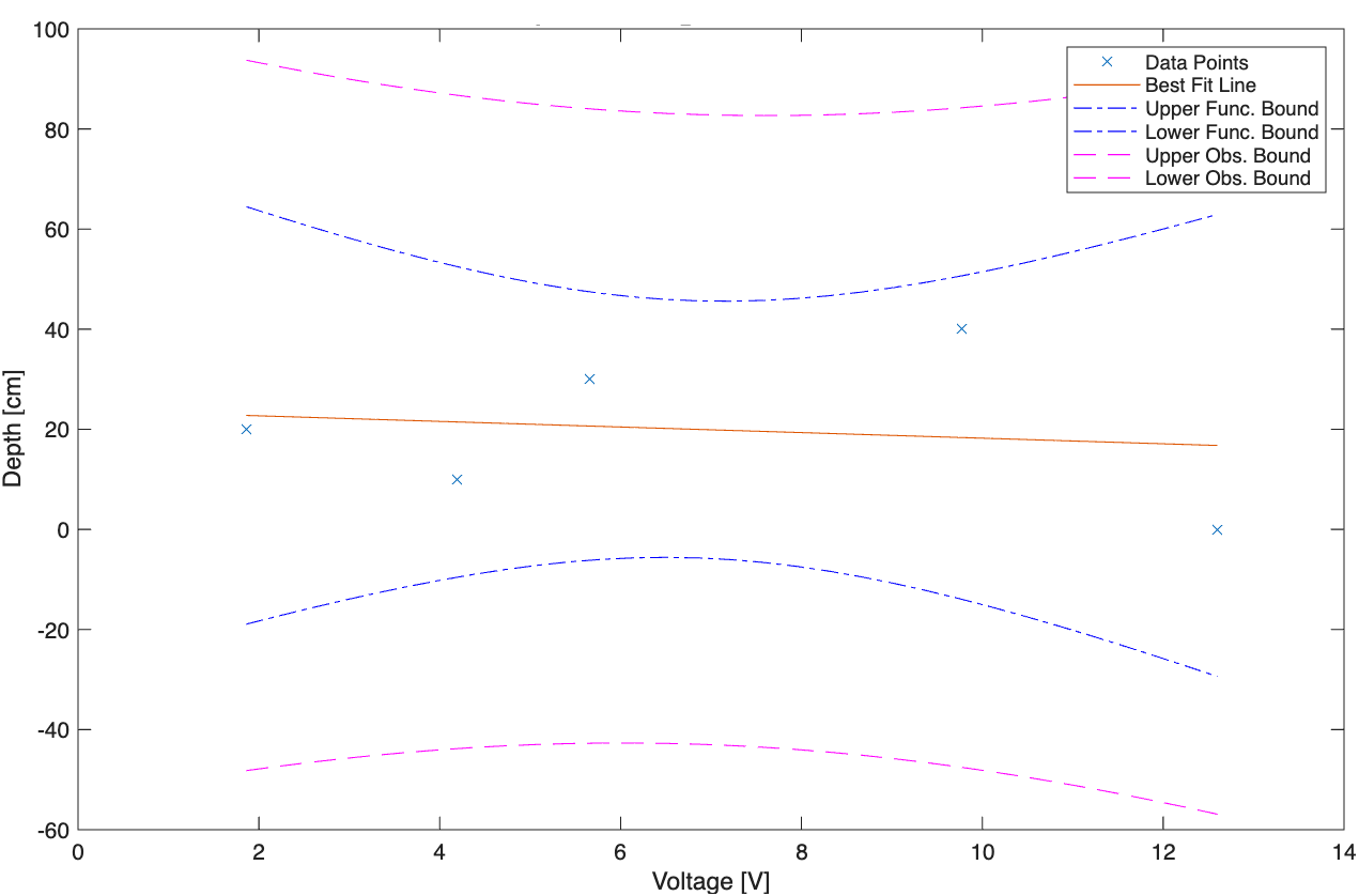
There is some percent error between the predicted and measured voltage outputs because the predicted values were calculated assuming each component (pressure sensor, op-amp, resistors, power supply, etc.) was ideal, but in reality, they all have errors in their values (resistance or output voltage). We also calculated the required resistors and thus output voltage with the assumption that the ambient pressure we recorded was accurate, and that it increased with depth according to Po+ρgh, where ρ = \(1000kgm^{-3}\), and g = \(9.81ms^{-2}\), but these values could have varied based on the barometer we used, the water we used, and the altitude. There are also errors associated with the multimeter reading for the voltage.
Temperature Sensors
There are three core temperature sensors, each with advantages and disadvantages. Each sensor was prototyped and tested to determine which would be the best fit for the project.
Thermistor
Thermistors change their resistance based on the temperature they are in contact with. The thermistor used was a NXFT15XH103FEAB035, and to convert the thermistor resistance to a Teensy 4.0 readable voltage, a voltage divider circuit was combined with an offset amplifier to shift and scale the output voltage so that temperatures from 0-20°C corresponded to voltages of 0.3-3V. This was calculated using the thermistor datasheet equation \(R=R_0e^{B(\frac{1}{T}-\frac{1}{T_0})}\) where the B-constant for 25°C/50°C is 4050K, \(R_0=47k\Omega\), and \(T_0=298.15K\), as well as voltage divider and offset amplifier calculations. Additionally, a unity gain amplifier was connected to prevent loading from the Teensy 4.0. The schematic of the thermistor circuit is shown in Figure x.
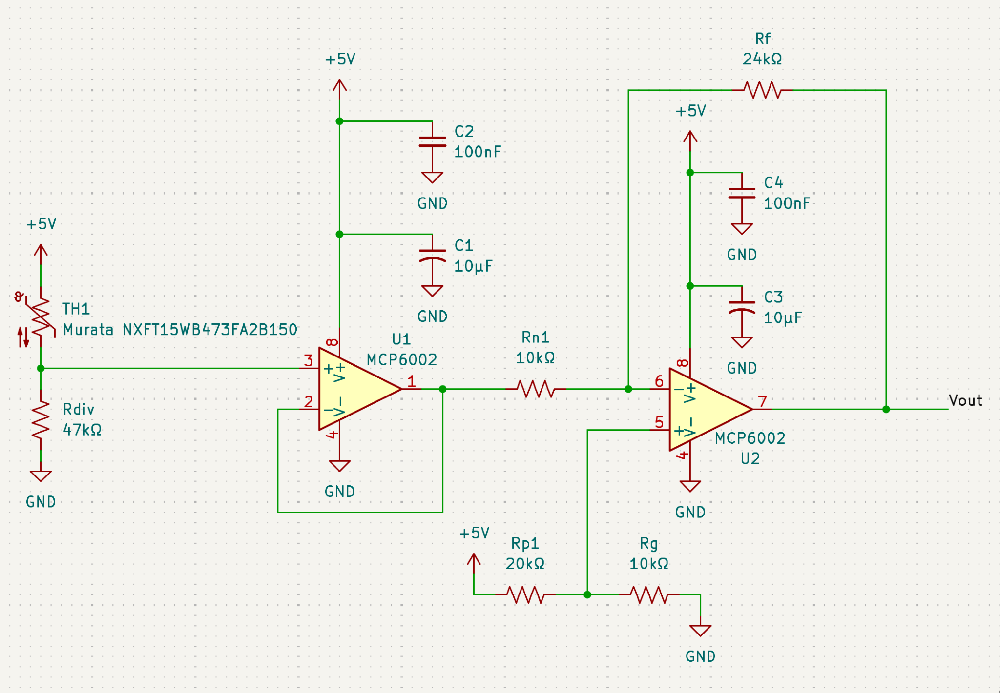
The thermistor was placed in approximately 0° and 20°C water baths, and the output voltage was measured with a multimeter. The results are shown in Table x.
Table 1. Thermistor Circuit Output Voltage and Resistance Measurements at 0°C and 20°C
| Temp (°C) | \(R_{predicted}\) (Ω) | \(R_{measured}\) (Ω) | \(V_{predicted}\) (V) | \(V_{measured}\) (V) | Error (%) |
|---|---|---|---|---|---|
| 0 | 162943 | 150.8k | 2.980 | 2.971 | 0.46 |
| 20 | 59254 | 56.9k | 0.359 | 0.300 | 2.93 |
There is a percentage error between \(V_{predicted}\) and \(V_{measured}\) values because the \(V_{predicted}\) values were calculated assuming each component (thermistor, op-amp, resistors, power supply, etc.) was ideal, but in reality, they all have errors in their values (resistance or output voltage). There are also errors associated with the multimeter reading for \(V_{measured}\) and added lead/contact resistance from where the thermistor was connected in the circuit, which would affect the output of the voltage divider. Further errors could come from the water temperature not being exactly 0°C or 20°C, even though they were measured to be this temperature by a digital thermometer. This is due to the thermometer measurement error, and the water temperature being non-uniform. The thermistor and digital thermometer cannot measure the exact same region of water, so they would not be reading the same temperature.
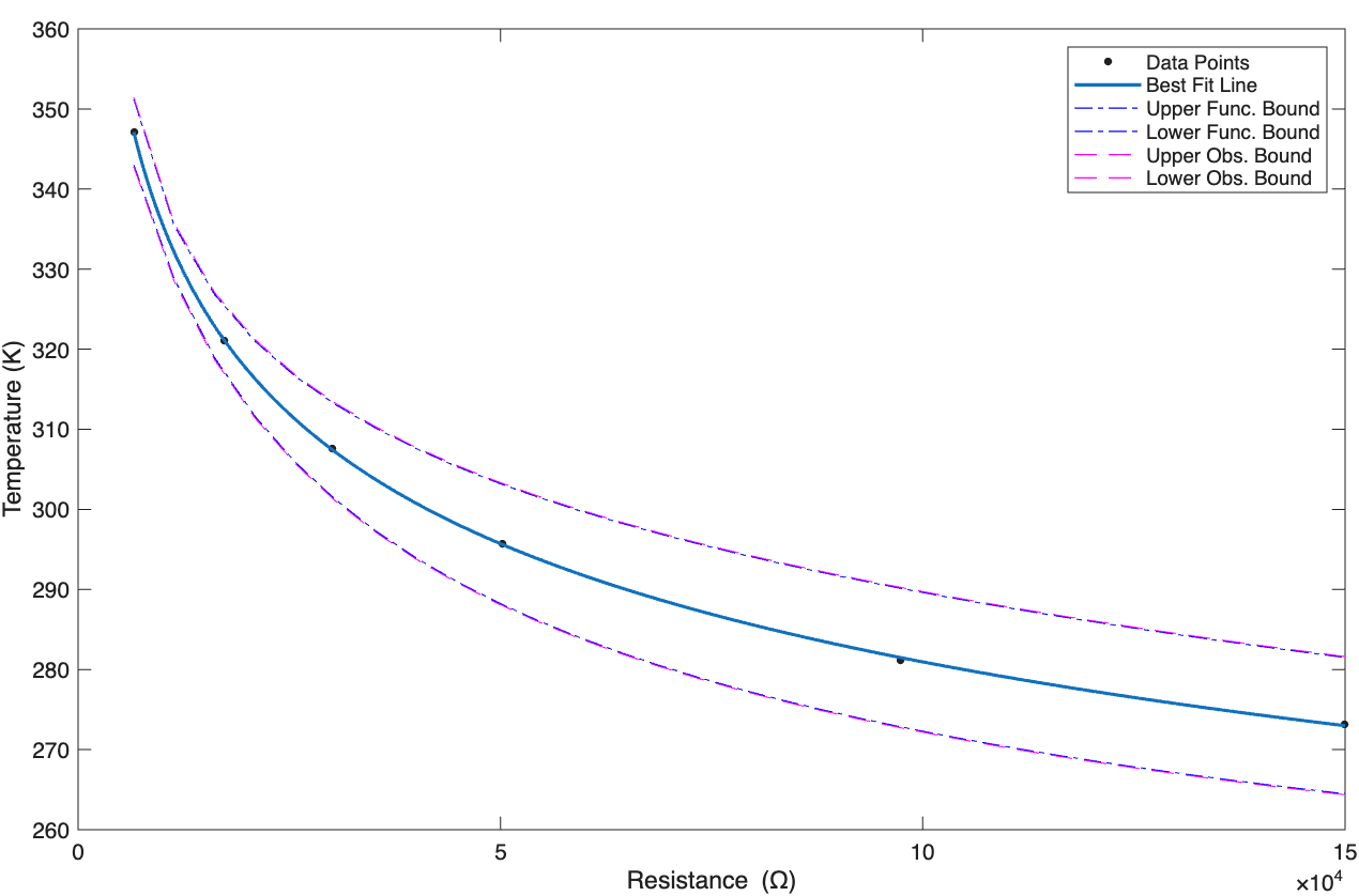
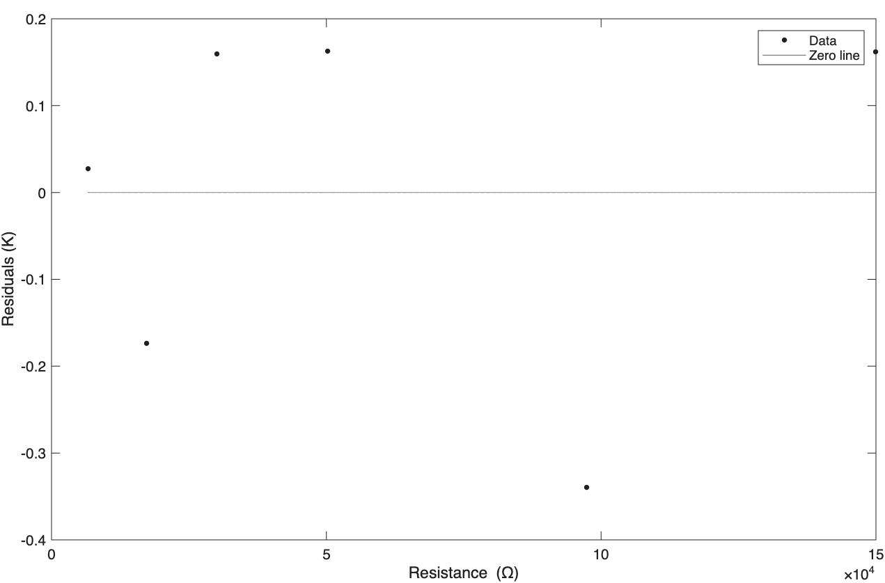
To relate the output voltage to temperature, the thermistor circuit was put in water baths ranging from 0-80°C, and the output voltage was measured with a multimeter. Using the circuit resistance values, the resistance of the thermistor was backsolved for each temperature. Then, using MATLAB, the Steinhart-Hart coefficients were calculated and a Steinhart-Hart fit was applied. The resulting plots are shown in Figure x.
Thermocouple
Thermocouples are temperature sensors that utilize the Seeback Effect (voltage is generated when two dissimilar metals are connected in a circuit and have junctions at different temperatures) to measure temperatures. The team experimented with a K-type thermocouple (chosen for easy measurement directly with a multimeter) to see if the temperature could be easily and accurately measured from the output voltage.
Using six water baths ranging from 0-80°C (measured with a digital thermometer), the bath temperature was measured using the thermocouple by putting the multimeter in temperature mode, and the thermocouple voltage was measured with a multimeter. Using the principles of cold-junction compensation (since the thermocouple cold junction is at the connection to the multimeter), the temperature could be decoded from the recorded voltage using NIST tables. The results are shown in Table x.
Table x. Thermocouple Measurement Results
| \(T_{thermometer}\) (°C) | \(T_{thermocouple}\) (°C) | \(V_{thermocouple}\) (mV) | \(V_{cold junction compensation}\) (mV) | \(T_{decoded}\) (°C) |
|---|---|---|---|---|
| 0.2 | -1 | -0.74 | 0.0178 | 0 |
| 8.9 | 8 | -0.41 | 0.3478 | 9 |
| 22.6 | 21 | 0.1 | 0.8578 | 21 |
| 34.6 | 34 | 0.62 | 1.3778 | 34 |
| 52.8 | 50 | 1.36 | 2.1178 | 52 |
| 72.7 | 70 | 2.17 | 2.9278 | 72 |
\(T_{thermometer}\) and \(T_{thermocouple}\) do not exactly match because the digital thermometer has errors associated with its reading (affecting \(T_{thermometer}\)), and the multimeter has independent errors associated with its reading (affecting \(T_{thermocouple}\)). Also, the temperature in the bath was likely non-uniform, and the thermocouple and digital thermometer cannot measure exactly the same point in the water, which contributes to discrepancies between them. In addition, the thermocouple measurements depend on cold junction compensation (even though the multimeter essentially does the NIST lookup), and any difference between the multimeter’s assumed cold-junction temperature and the true junction temperature introduces systematic error.
Integrated Silicon Linear Sensor
The IC sensor required no special circuitry besides wiring up \(V_{DD}\), \(V_{OUT}\) and GND. Since the output voltage is linearly dependent on temperature with an equation in the datasheet, there was no calibration necessary.
Comparing the Sensors
The settling time of the three temperature sensors were compared. Each sensor was directly connected to a multimeter and dipped in a ~0°C bath until the output reading was stable, then transferred to a ~80°C bath. The time it took for the reading to stabilize was recorded. The K-type thermocouple had the fastest settling time of 2.62s, the thermistor had a medium settling time of 16.79s, and the IC sensor (MCP9701A) had the slowest settling time of 42.49s.
Since the thermocouple had the fastest settling time, the team thought it could be a good option for the AUV, especially if the AUV would be travelling at high speeds and need near-immediate temperature readings. However, it would need a second temperature sensor to measure the cold junction temperature as it would be unrealistic to keep it at a constant temperature while the AUV is deployed.
The thermistor was also seen as a good option for the AUV because its settling time was still pretty fast, and it would be easier to integrate with the AUV. It also gave more accurate readings than the thermocouple, and even though it had a smaller temperature range than the thermocouple the AUV would not be going in regions that exceeded its limits.
The IC sensor was not considered because its settling time was too slow, even if the AUV were just drifting in water.
Underwater Acoustics
Acoustics are helpful for a variety of sensors, such as sonar and radar. To investigate the feasibility of underwater acoustic measurements, the team used acoustic measurements to locate relative position in a tank with multiple speakers emitting set frequencies.
Getting Familiar With Signal Processing Using Fast Fourier Transforms
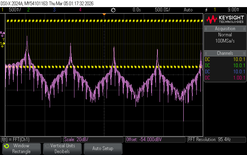
Fast Fourier Transforms were applied using the FFT function of an oscilloscope to 11kHz and 12kHz sine and square waves with 1.5V amplitude and 0V offset.
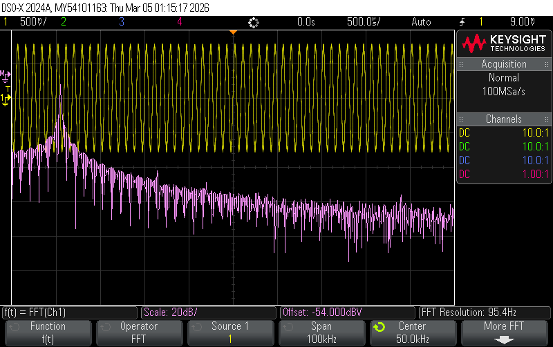
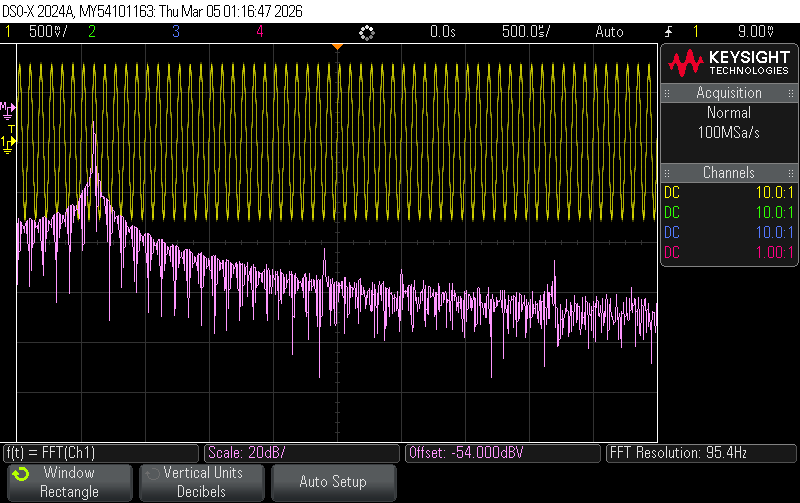
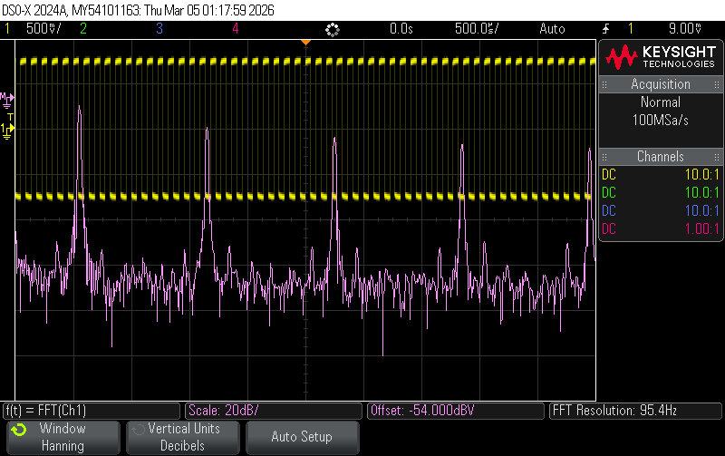
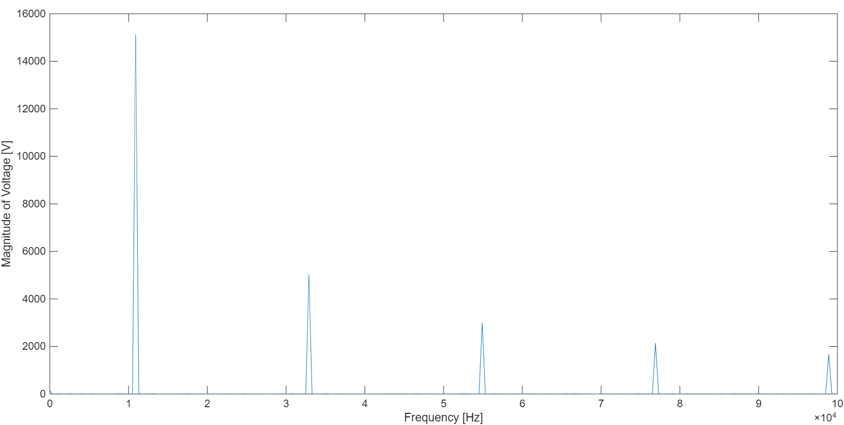
The plots of FFT magnitude show the amplitude of frequencies in the signal. Since Figure Xa shows a 11kHz sine wave and its FFT, we see a single peak at 11kHz, whereas Figure Xb shows a 12kHz sine wave and its FFT, so we see a single peak at 12kHz.
Figure Xc shows a 11kHz square wave and its FFT, and since a square wave can be represented by the sum of sine waves with odd integer multiples of frequencies, we see multiple peaks, each at an odd integer multiple of 11kHz.
The unit step function is given by: \[ \begin{aligned} U(x)&=0 \text{ (for }x<0)\\ U(x)&=\frac{1}{2} \text{ (for }x=0)\\ U(x)&=1 \text{ (for }x>0)\\ \end{aligned} \]
A square wave with period \(T=2L\) can be expressed as \(f(t)=2(U(\frac{t}{L})-U(\frac{t}{L}-1))-1\).
The Fourier Series representation of this signal is:
\[ \begin{aligned} f(t)&=a_0+\sum_{k=1}^{\infty}a_kcos(kw_ot)+\sum_{k=1}^{\infty}b_kcos(kw_ot)\\ &=a_0+\sum_{k=1}^{\infty}a_kcos(k\frac{\pi}{L}t)+\sum_{k=1}^{\infty}b_kcos(k\frac{\pi}{L}t)\\ \end{aligned} \]
Since the square wave is an odd function, \(a_o=a_k=0\). Solving for \(b_k\):
\[ \begin{aligned} b_k&=\frac{2}{T}\int_{0}^{T}f(t)sin(k\frac{\pi}{L}t)dt\\ &=\frac{1}{T}\int_{0}^{2L}f(t)sin(k\frac{\pi}{L}t)dt\\ &=\frac{2}{n\pi}(1-(-1)^n)\\ \end{aligned} \]
Which gives \(b_k=\frac{4}{n\pi}\) for odd integers k or \(b_k=0\) for even integers k.
Therefore, the sum of sines representation of a square wave is \(f(t)=\sum_{n=1,3,5,...}^{\infty}\frac{4}{n\pi}sin(2\pi nft)\).
Since n is a positive odd integer, and we take the sum of the function from n to infinity, the frequency peak locations would be equal to nf = positive odd integer multiples of 11kHz. This is why we see them present at 11, 33, 55, 77, 99 kHz (the x-axis only goes up to 105Hz). If the x-axis extended further, the magnitude of the peaks would eventually become so small that we wouldn’t be able to see them anyway. As more n-terms (and thus frequencies) are included, the sum of sines representation of the square wave gets closer to the shape of a perfect square wave.
Figure Xd also shows a 11kHz square wave, but with a Hanning window applied, and this eliminates the peaks at the non-odd integer multiples of 11kHz due to the Hanning window removing the periodic discontinuities and additional sinusoid component additions to compensate for them.
Figure Xe shows a MATLAB-generated plot of the frequency spectrum of the same signal in Figure Xd. The FFT peak positions match between Figures Xe and Xd, but the magnitude of the peaks is different because the y-axis of the oscilloscope plot is in decibels, while the y-axis of the MATLAB plot is in volts.
Fourier transformations expect all data that is put into it to be periodic, but the collected data is unlikely to be cut off at exactly a period of the real signal, so after the Fourier transform extends the collected data by repeating what is given to it, the FFT algorithm will think there is a periodic discontinuity and add a bunch of high frequency sinusoids to account for the mismatch. Multiplying the data by a windowing function makes sure the data goes to 0 at the sides of the window, and this removes any periodic discontinuities when the signal is repeated. Using a rectangular window would be like using no window at all since the whole signal is multiplied by a constant, so it has an assumed periodic discontinuity, and the Fourier transform will add many high-frequency sinusoids to compensate, whereas using a Hanning window would make the data at the sides of the window go to 0, removing the need for these undesired sinusoids.
Detecting AUV Position Using Acoustics
To pick up underwater audio signals, the team built a waterproof electret microphone circuit using op-amps.
The gain-bandwidth product is given by \(GBWP=f\times g\), where f is the bandwidth and g is the gain. The gain of the circuit would be limited by the gain from this equation at a certain frequency. Since the output of the microphone is very small (~10mV depending on the input), it needed to be scaled to be readable on an oscilloscope. This was done with two non-inverting amplifiers with a gain of 10 in series. The specific op-amp used was chosen by comparing their tolerant frequencies that would allow for this gain.
The OP07 op-amp has a GBWP of 0.6MHz. Using the GBWP equation with a gain of 10, the OP07 will have ideal op-amp behaviour and allow for a gain of 10 for frequencies up to 60kHz. The bandwidth of the OP07 at each stage is 60kHz with a gain of 10.
The TL081 op-amp has a GBWP of 4MHz. Using the GBWP equation with a gain of 10, the TL081 will have ideal op-amp behaviour and allow for a gain of 10 for frequencies up to 400kHz. The bandwidth of the TL081 at each stage is 400kHz with a gain of 10.
The frequencies we used the microphone with were within both these ranges, so using either op-amp was feasible. The TL081 was chosen since it can amplify a wider frequency range. The schematic for the microphone circuit is shown in Figure x.
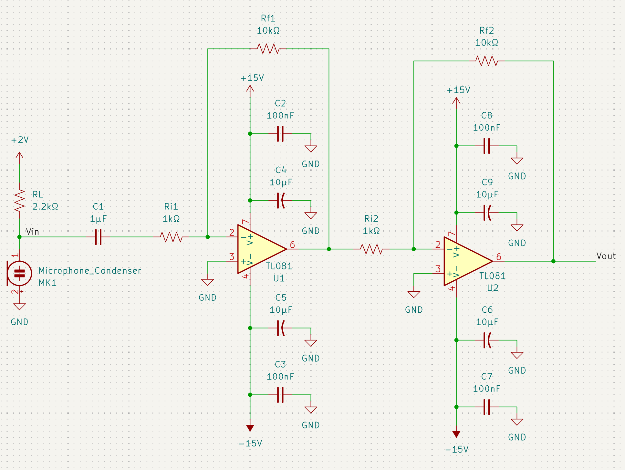
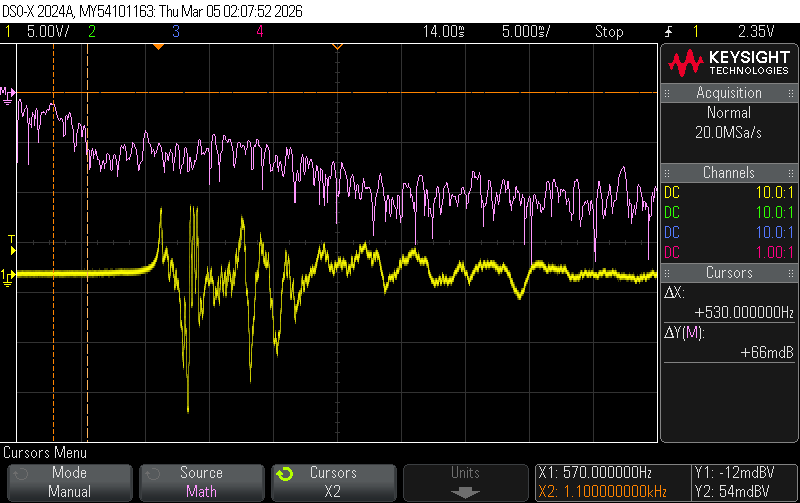
The circuit was tested by reading the output using an oscilloscope while someone clapped (shown in Figure x). The oscilloscope internal FFT function showed that the hand clap has frequencies from 570Hz to 1.1kHz, which are all within the human audible frequency range, which makes sense because we can hear hand claps.
After testing, the microphone was placed in water close and facing to each beacon. Figures Xa-c show the oscillloscope traces obtained.
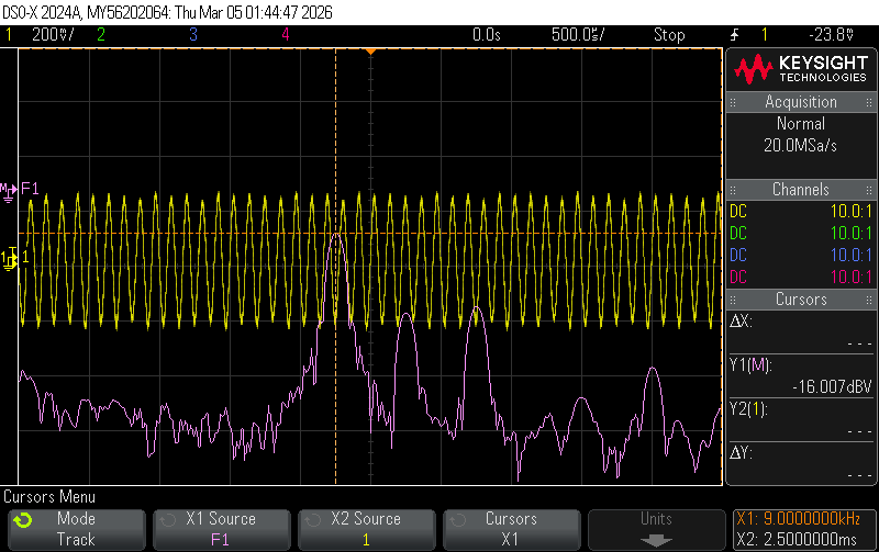
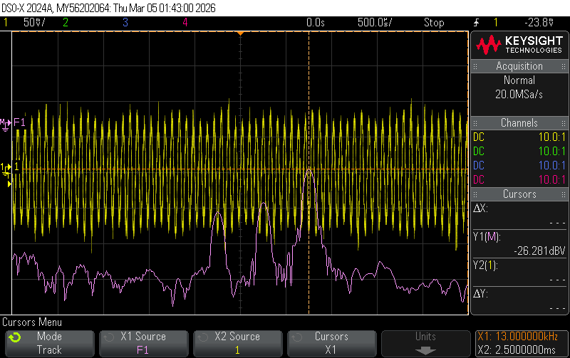
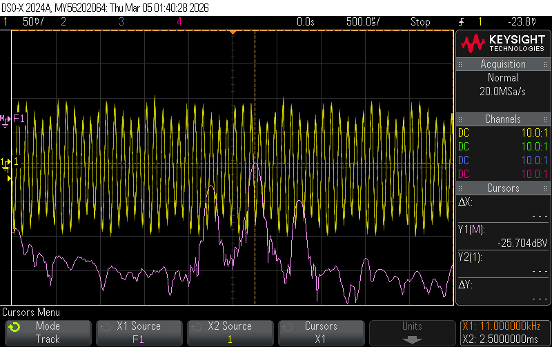
The frequency each beacon was emitting was observed through the highest magnitude FFT frequency read off the oscilloscope when the microphone was next to that beacon. The emitted signal could be recreated by sampling at various distances away from the beacon.
Each beacon emits a signal travelling in the forward direction (call this \(P_F\) and represent it as sinusoid multiplied by the power transmitted by the speaker \(P_0\)), and this gets reflected off a wall in the tank so it travels in the reverse direction (call this \(P_R\) and represent it as a sinusoid multiplied by the power transmitted by the speaker \(P_0\)), which creates [at least 1] multipath. These are functions of time (t), and \(t=0\) since we observed a snapshot in time, and we want to know their amplitude at a certain distance away from the source (x), so that we can sum them and get the power the microphone receives.
\(P_F=P_0Re(e^{i(t+2\pi fx)}=p_pRe(e^{i2\pi fx}\) and \(P_R=P_0Re(e^{i(t-2\pi fx)}=p_pRe(e^{-i2\pi fx}\)
Thus, \(P_{total}=P_F+P_R=2P_0cos(2\pi fx)\).
The spatial wavelength is the speed of sound in water (\(~1500ms^{-1}\)) divided by the frequency emitted by the beacons (f = 9kHz, 11kHz, 13kHz), which gives λ=16.67, 13.64, 11.54cm (this is the distance between when each wave will start repeating). From Nyquist-Shannon Sampling theorem, we need to sample at least twice the maximum frequency emitted by the beacons to observe the correct signal, so we get that the x-axis spacing needs to be 5.77cm. To be safe, samples were taken closer together at 2cm apart since because the ideal behaviour assuming one multipath will likely not occur.
Figure X shows the collected voltage magnitudes when the microphone was held at various distances away from beacon 1 overlaid onto a line of typical magnitude decay behaviour. The collected data points do not exactly line up with the decay because they show a sinusoidal function decaying over time, which lines up with the emitted signal.
Experimenting with Sample Rates
Using an additional offset amplifier, the microphone circuit was connected to the Teensy 4.0 to sample data. Putting the microphone inside the tank, the first 100 data points of time-scale data and the magnitude of FFTs when sampling at 10kS/s and 100kS/s were plotted, as shown in Figures Xa-d.
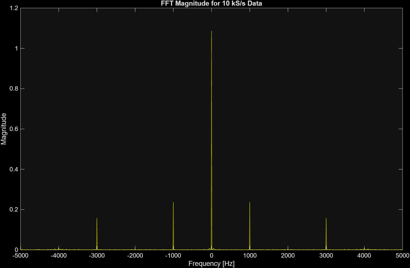
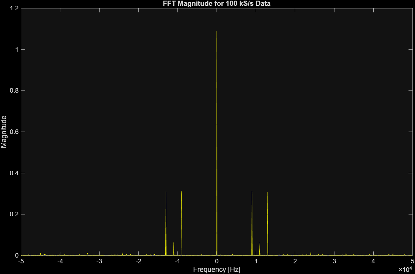
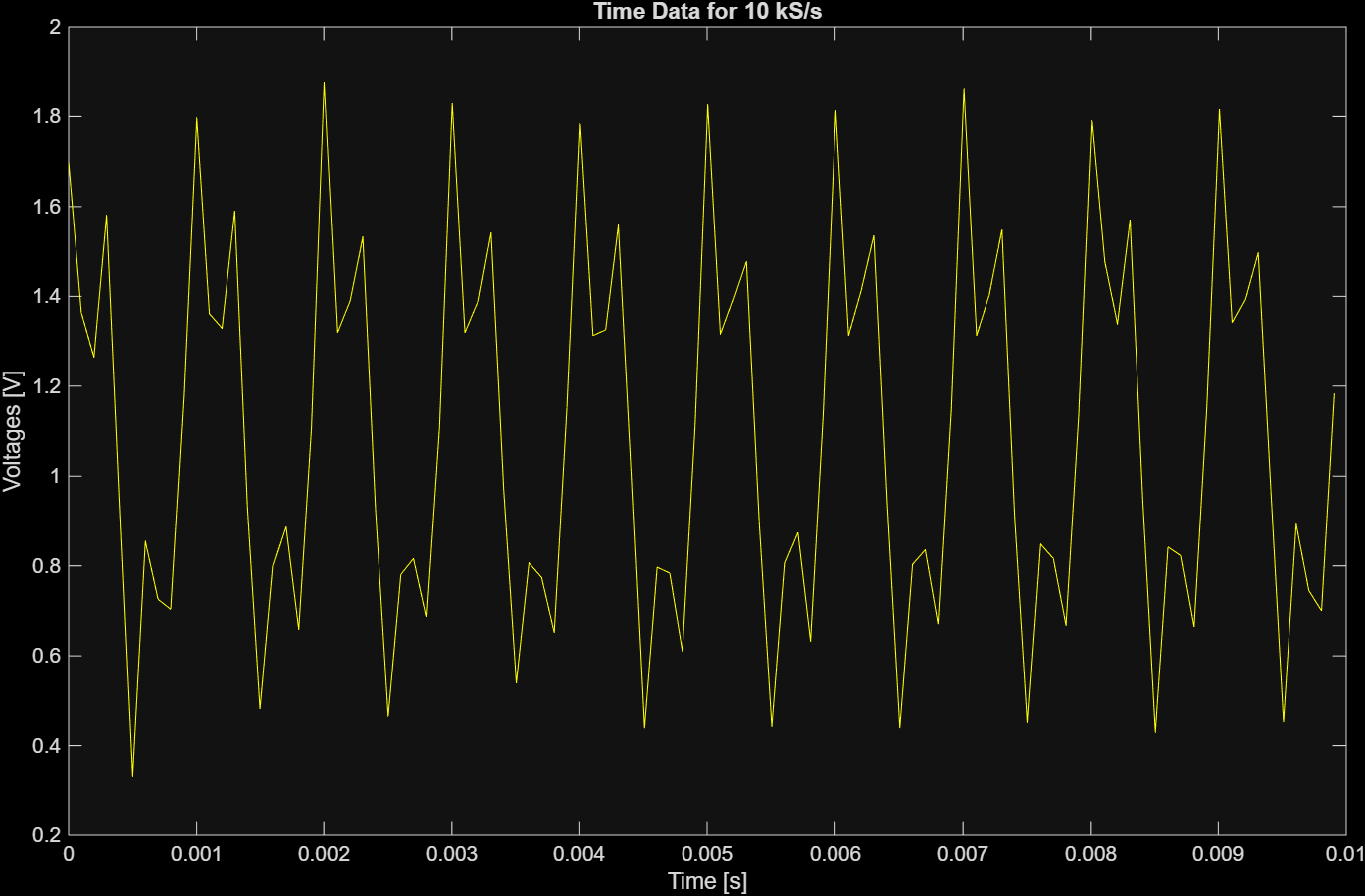
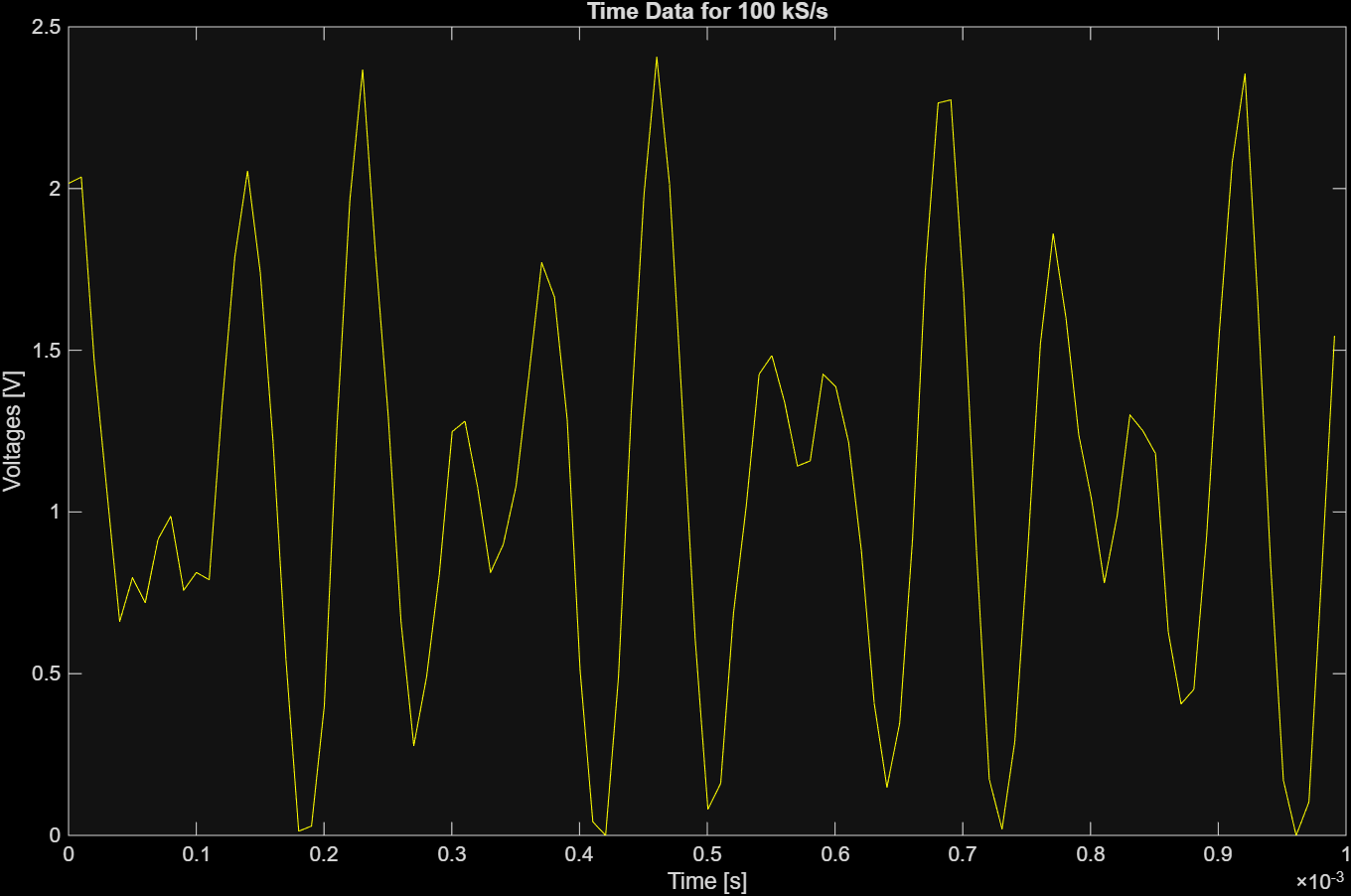
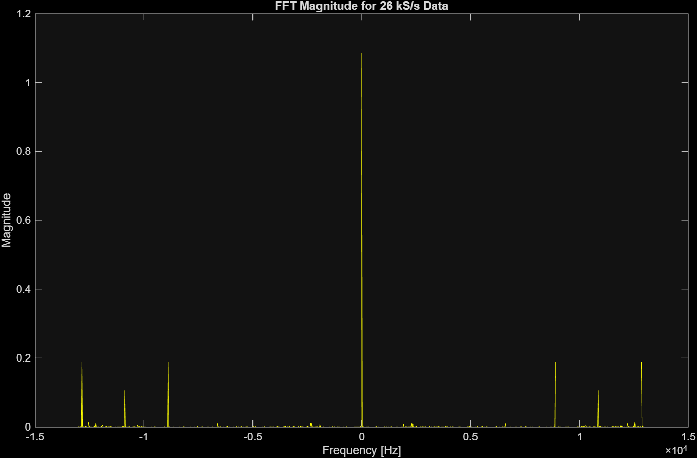
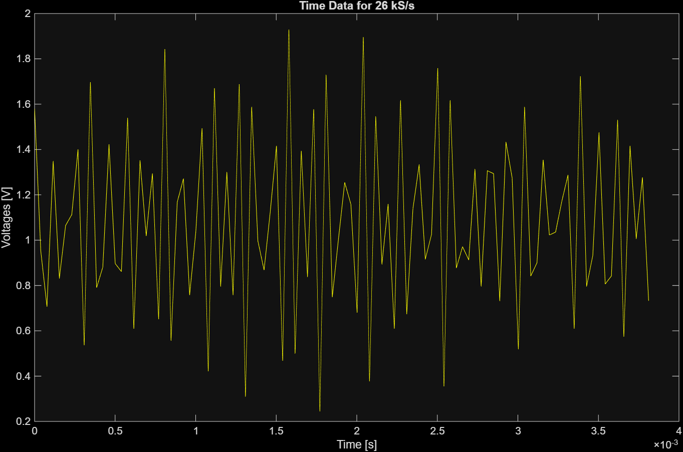
The FFT plots show different frequency magnitude peaks and the time data plots show different sinusoidal behaviour. This is because the maximum transmitted frequency of the sine waves in the tank was 13kHz. From Nyquist-Shannon Sampling theorem, to observe total signal, we need a sampling frequency greater than twice this frequency, so 26kHz or higher. So the 100kS/s (units equivalent to kHz) sampling rate would be enough to fully observe the wave, whereas using the 10kS/s sample rate would result in aliasing. This explains why the data seen in the 100kS/s plots matched the frequencies in the tank whereas the data we see in the 10kS/s plots shows frequencies smaller than expected.
Figures Xa-b show the FFT magnitude plot and time-scale plot when sampling at 26kS/s. They show correct frequency peaks and superpositioned waveform.
Magnetometer
The team chose to use a magnetometer to collect magnetic flux density readings on the ocean floor. Magnetic flux density is a quantity that describes the magnitude of a magnetic field. Ferromagnetic materials induce magnetism and change the magnetic field around them when they are placed in an external magnetic field. The Earth has a magnetic field that is downward-angled in the northern hemisphere (which includes the deployment site: Dana Point, CA). Thus, ferromagnetic materials in the deployment area would increase the magnetic flux density around them. This change in magnetic field decreases according to the inverse cube of distance. Magnetic flux density is highly dependent on material composition and object size, and these quantities of the underwater debris were unknown. Therefore, the PNI RM3100 sensor, which converts changes in sensor inductance to magnetic flux density readings, was chosen to detect ferromagnetic materials because of its large range (-800 to 800µT), low noise (15nT), and high sensitivity.
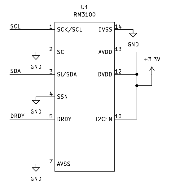
The magnetometer had both I2C and SPI connection protocols. Since the team did not need particularly high speed data readings (readings would only be taken at the sea floor) and did not need to send at receive data at the same time, the I2C protocol was used. The relevant pins were connected to the Teensy 4.0 as shown in Figure x.
Its functionality was confirmed by holding various magnets at different distances away from it and observing the change in magnetic flux density readings.
Modifications to the Circuits for Deployment
To prepare the sensors for deployment at Dana Point, the pressure sensor and thermistor circuits were modified to more appropriately scale their predicted output range to the input range of the Teensy 4.0.
Sensor Justification
The thermistor was chosen over the IC sensor and thermocouple because of its fast response time, higher sensitivity, very low effect of lead resistance on accuracy, and ease of linearising its non-linear relationship between output resistance and temperature.The NXFT15XH103FEAB035 thermistor was chosen to collect temperature data because of its large operating temperature range (-40-125°C), high accuracy (±1% resistance), and easy integration with the AUV.
The team decided that temperature and pressure sensors would be suitable for this project’s goals because the concept of geostrophic balance would help us back-calculate debris drop locations.
Geostrophic balance describes the state of fluid flow (currents) in the ocean based on a steady-state force balance between the pressure gradient in the ocean (which is influenced by factors such as surface winds) and the apparent force on particles moving in the water relative to the Earth’s rotating reference frame. The velocity of fluid particles along the Cartesian x and y axes is related to the fluid density, Earth’s rotation rate, and the latitude of the particle. Flows in the ocean occur along lines of equal pressure, so there would be a different set of current vectors at each measured depth. The density of seawater changes throughout the ocean based on the One Atmosphere International Equation of State of Seawater, which is dependent on temperature and salinity. Salinity of ocean water is roughly constant over 10-100m of depth and along the ocean surface. However, temperature in the ocean changes rapidly (10-20°C fluctuation) over the first 400m deep into the ocean, especially in mid-latitude regions (including California). Thus, to characterize oceanic currents according to the above, pressure and temperature readings were collected at various points in the ocean.
Pressure Sensor
The MPX5700 outputs voltages that are linearly related to absolute pressure. It was expected that the pressure sensor would output voltages of 0.85-1.04V corresponding to depths of 0-3m below the ocean’s surface. The 0-3m range was chosen because Dana Point Harbour has depths between 6-15ft (1.83-4.57m), and the deployment locations were in shallower regions with a 0-3m range. As shown in Figure X, the offset amplifier (U3) was modified to scale this output to nearly fill the 0-3.3V input range of the Teensy 4.0 microcontroller to maximize data resolution. A unity gain buffer (U2) was placed between the pressure sensor and offset amplifier to prevent loading effects.
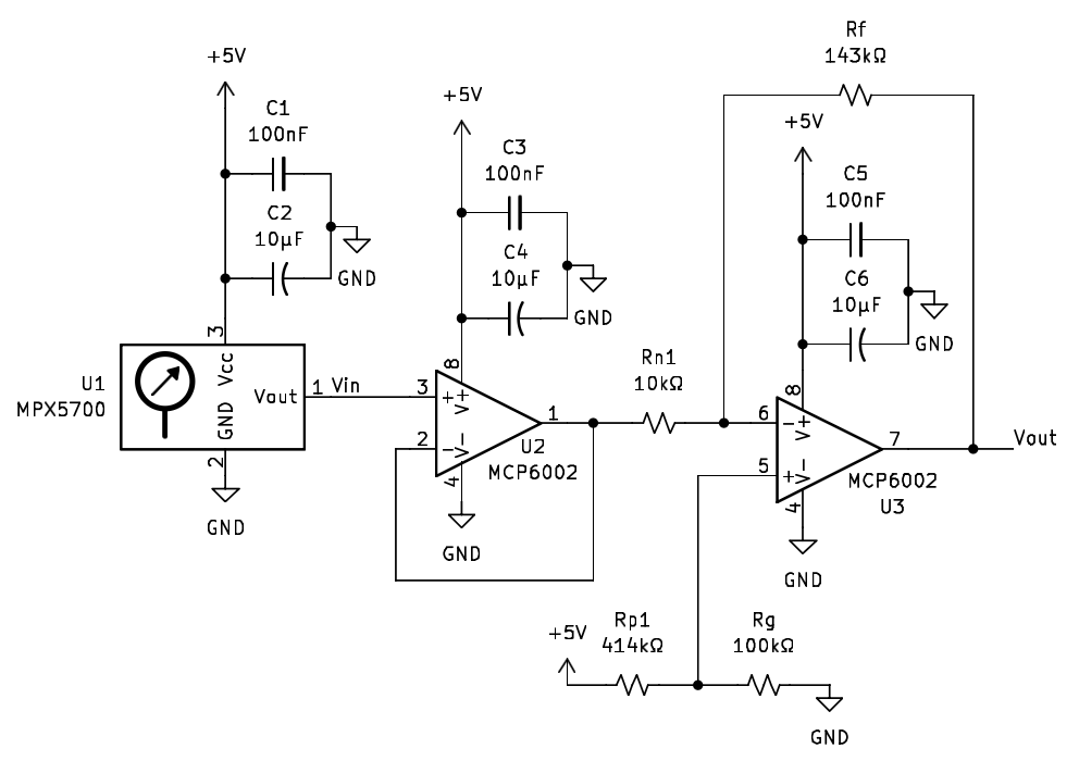
The offset amplifier was designed with an offset of 14.56V and a gain of -14, calculated using the offset amplifier equation \(V_{out}=5\left(1+\frac{R_f}{R_{n1}}\right)\left(\frac{R_g}{R_{p1}+R_g}\right)-\frac{V_{in}R_f}{R_{n1}}\label{eq}\). The variable values in this equation for this circuit are as depicted in Figure X. This resulted in theoretical output voltages of 0.01-2.73V for depths 3-0m, which is within the desired range. A small voltage buffer was left on each side of the output to ensure fluctuations from noise and unanticipated depths slightly outside the expected range would not cause the circuit to rail out.
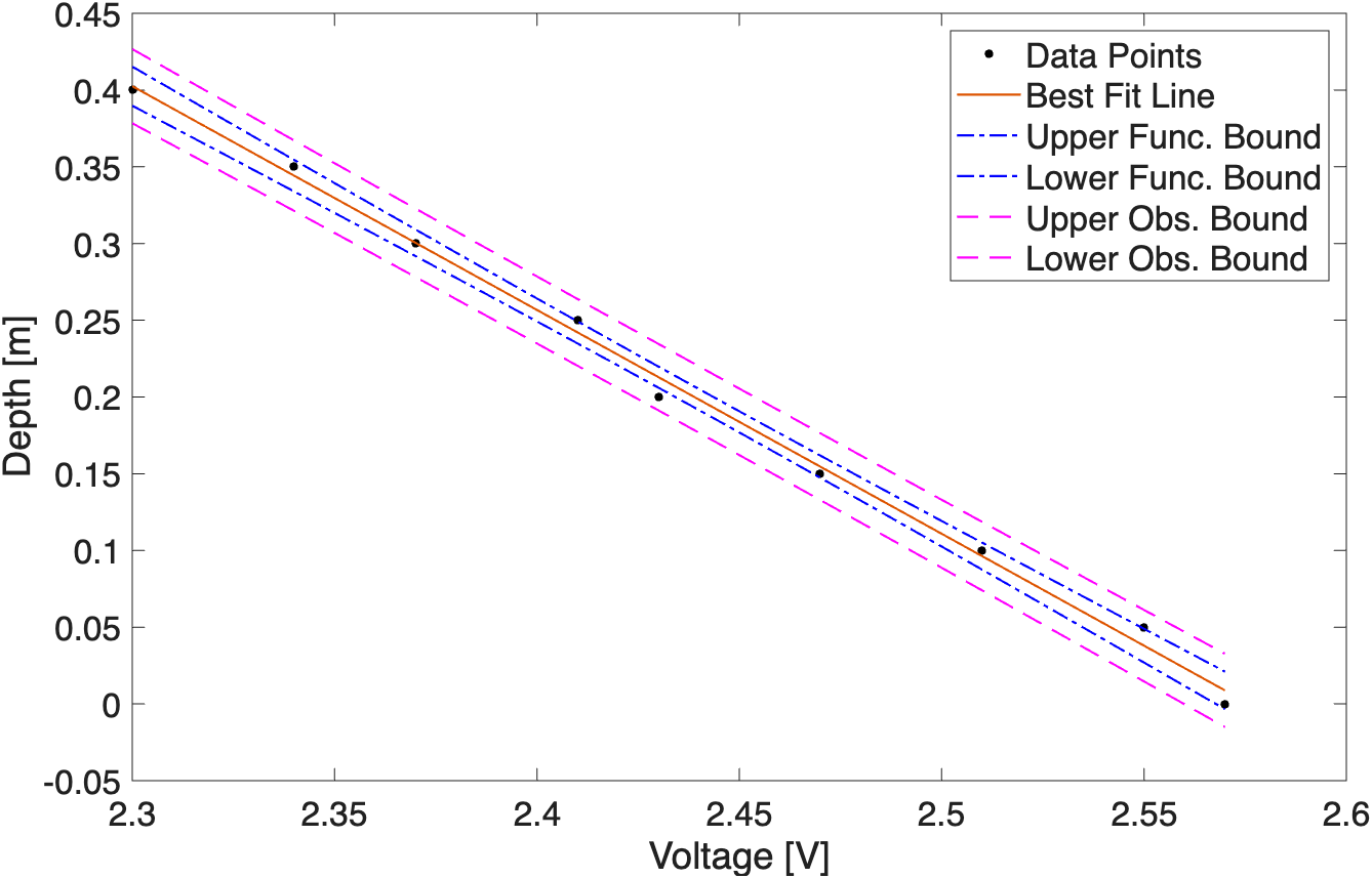
The output of the pressure sensor is DC voltage, so the 10Hz sampling frequency in the code was sufficient. However, as described in the P-control section, the depth control algorithm was modified to allow the AUV to autonomously determine if it had reached the seafloor to isolate magnetometer readings at the bottom of the ocean. The sensor was calibrated to derive an equation relating the output voltage to depth by taping a pressure tube connected to the pressure sensor to a meterstick. The output voltage of the circuit was recorded while holding the end of the tube at depths from 0-0.4m in increments of 0.05m in a graduated cylinder filled with seawater. Figure X shows the resultant calibration curve with 95% confidence level upper and lower observational and functional bounds. The \(R^2\) value for the fit was 0.996. After calibration, it was noted that the maximum depth that could be recorded was 3.76m under the surface of the water, which was outside the planned 0-3m range.
Thermistor
The NXFT15XH103FEAB035 changes its resistance based on its contact temperature. From its datasheet, thermistor resistances of 95420-47000 \(\Omega\) were expected for temperatures of 10-25°C, which is the approximate ocean temperature at Dana Point in April with a 2-5°C buffer on each side. As shown in Figure X, a voltage divider was created with the thermistor to convert this output resistance to an output voltage. A unity gain buffer and offset amplifier were then used to scale this output to 0-3.3V in the same way as the pressure sensor. The voltage divider equation is \(V_{in}=\frac{5R_{div}}{R_t+R_{div}}\), with the variable values as depicted in Figure X.
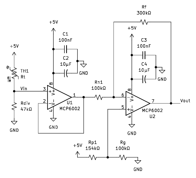
The offset amplifier was designed with an offset of 12.13V and a gain of -3. This resulted in theoretical output voltages of 0.37-2.95V for temperatures 25-10°C, which is within the desired range. Like the pressure sensor, the voltage buffer on each side of the output prevents railing out during deployment.
The output of the thermistor interface circuit is DC voltage, so the default 10Hz sampling frequency in the code was sufficient, and no software modifications were made.
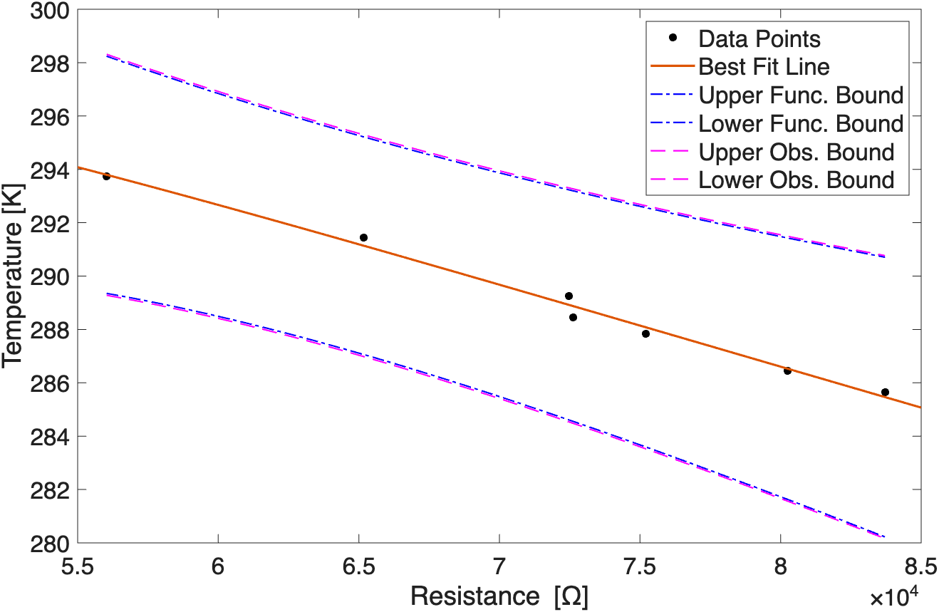
The thermistor resistance is related to temperature based on the Steinhart-Hart equation, where T is the temperature in K, R is the thermistor resistance in \(\Omega\), and A, B, C, and D are unitless Steinhart-Hart coefficients. As shown in Figure X, the thermistor was calibrated by measuring output voltages when placing the thermistor in 10-25°C water baths, backcalculating the thermistor resistance using, and finding the Steinhart-Hart coefficients. The coefficients with 95% confidence bounds were found to be A=0.02348 (-0.1563, 0.2032), B=-0.005701 (-0.05414, 0.04274), C=5.159 \(\times10^{-4}\) (-0.003816, 0.004848), and D=-1.487 \(\times10^{-5}\) (-1.424×\(10^{-4}\), 1.127×\(10^{-4}\)). Combining the offset amplifier equation and Steinhart-Hart equation determined the relationship between output voltage and temperature.
Magnetometer
The magnetometer interface circuit was not modified after the I2C connection (Serial Clock (SCL), Serial Data (SDA), and Data Ready (DRDY) lines) was tested to work.
The default 10Hz sampling frequency in the code was sufficient for the magnetometer readings. The magnetic flux density was expected to be a roughly constant value at each position, and not a periodic signal, so the sampling frequency producing aliasing was not a concern. Separately, the RM3100 has a data update rate of 37Hz, meaning it would complete a measurement and flag DRDY every 0.027s [13]. If the sampling frequency were more than 37Hz, the Teensy 4.0 could attempt to read data when there is no real output, producing gaps or anomalous values in the recorded data.
Modifications to the code were made in the form of writing C++ functions and constants necessary for the magnetometer to collect and save separate-axis and total magnitude magnetic flux density readings in µT.
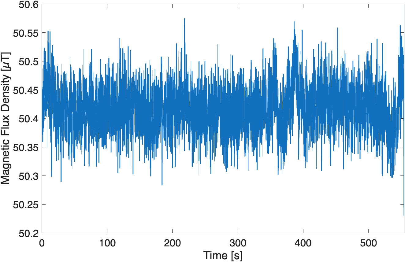
The sensor was re-validated before deployment by using it to collect data in open air and away from any ferromagnetic objects (apart from data collection hardware) for around 10 minutes. Figure X shows the results of this data collection, where readings fluctuated between around 50.25-50.6µT, which falls within the expected range of 22-67µT on the Earth’s surface.
Mechanical Design: Buoyancy and Waterproofing
The AUV was designed to be a diving and surface AUV which would autonomously use P-control to travel to a selected waypoint on the surface of the water located through a GPS. It would then use P-control to dive to selected depth waypoints, stopping at each one for five seconds to take measurements of temperature and magnetic flux density until it either reached the maximum set depth of 3.5m or the sea floor. It would then surface and navigate to a set location for collection.
As shown in Figure X, the AUV was shaped as a rectangular prism with two z-direction motors for diving and two xy-direction motors for surface navigation attached along the center horizontal axis. A waterproof box enclosing a Teensy 4.0, Inertial Measurement Unit (IMU), Global Positioning System unit (GPS), motor drivers, a microSD card with a reader, and the sensor circuits was placed on the top of the AUV. The magnetometer sensor was enclosed in a separate waterproof box at the bottom of the AUV. This was done to maximize the distance between the motors, the magnetometer sensor at the bottom of the AUV, and the magnetometer integrated in the IMU at the top of the AUV, such that the motors have limited interference with each of the magnetometer’s readings. The pressure sensor tube was fixed along the side of the AUV such that it ended at a point level with the motors, so that when the z-direction motors drove upwards at maximum speed, the pressure tube would end at the surface of the water. The thermistor was fixed along the other side of the AUV such that its head was at the same level as the pressure sensor tube end to take measurements at the same depth.
The waterproof boxes were adapted to fit all wires and the pressure tube using penetrator bolts coated with marine epoxy. The top box had five penetrator bolts to hold the pressure tube, 2 wires for the thermistor, 2 wires for each of the 4 motors, and 6 wires for the magnetometer ground, power, and data lines. The bottom box had two penetrator bolts to hold the 6 magnetometer wires, and the ground and power wires were later split to accommodate the necessary pins. All sensors were waterproofed to prevent shorts in the water by heat-shrinking any exposed solder connections.
The AUV was designed to be approximately neutrally buoyant so that the z-direction motors could generate enough thrust for both descending and ascending in the water. The AUV had a total mass of 2.45kg. Using the equation for buoyancy force \(F_b=\rho Vg\) , where \(F_{b}\) is the buoyancy force of an object in N, \(\rho\) is the density of fluid the object is in in \(kgm^{-3}\), V is the object volume in \(m^3\), and g is the gravitational acceleration in \(ms^{-2}\), the total buoyancy force from all components such as the waterproof boxes, pool noodles, and motors on the AUV was 41.80N.
To make the AUV neutrally buoyant, the force of gravity had to be roughly equal to the buoyancy force. The mass of ballast that needed to be added to the AUV to achieve this was calculated using \(m_{ballast}=\frac{F_b}{g}-m_{AUV}\), where \(m_{ballast}\) is the required mass of ballast in kg, \(F_b\) is the total buoyancy force on the AUV in N, g is the gravitational acceleration in \(ms^{-2}\), and \(m_{AUV}\) is the total mass of the AUV in kg. By calculation, ballast weighing around 1.8kg was needed. However, after adding this, the AUV was slightly positively buoyant at the test deployment site pHake Lake, so a total of around 2kg of ballast was used. After this addition, the AUV was also positively buoyant at Dana Point due to the higher density of saltwater versus freshwater, so a total ballasting weight of 2.4977kg was used.
By symmetry, the center of buoyancy and mass of the AUV were along its center z-axis. Due to last-minute changes to the AUV, the center of buoyancy was 30.48cm from the top of the AUV, and the center of mass was 18.43cm from the top of the AUV. Since the center of buoyancy was below the center of mass, the AUV was not stable in the water. However, it still had a limited risk of tipping over because the waves at Dana Point were not strong enough to push the AUV past its restorative balancing point.
P-Control
Depth Control Algorithm
A P-control algorithm was programmed in C++ such that the AUV could traverse to a set of waypoints (hardcoded z-directions) and stay at each one for a set amount of time. This was done by tuning the Kp value, calculating the depth error (difference between desired and measured depth), and setting the motor control effort as a function of these two values. This was tested by having the algorithm run and observing the collected depths.
The algorithm was later modified so the AUV would self-determine if it had reached the seafloor by collecting a series of measurements and comparing the minimum and maximum output voltages. If the difference between these readings in a span of 20 seconds was less than 0.05V, the AUV would be at the seafloor and would surface. (Essentially some kind of comparative shift register!) Otherwise, if it reached the final waypoint instead, it would also surface.
Deployment
Deployment Procedure
A test deployment was conducted at pHake Lake, but no usable data was collected due to the Teensy 4.0 combusting from an internal short and a bug in the Arduino IDE code that caused a replacement Teensy 4.0 to reset every 5 seconds.
Deployments at Dana Point were conducted in the early morning to minimize human activity that could interfere with the AUV’s position while diving. Initially, it was planned that both surface and depth control would be used to deploy the AUV autonomously. However, the GPS readings were too unreliable to use surface control, as the readings would fluctuate on a scale of 5m, and the AUV refused to move past the first waypoint. Additionally, the GPS lock would be lost after diving and would take over 10 minutes to reconnect to satellites, so it would not be able to return to shore reliably. Only depth control was used for data collection.
At Dana Point, a new calibration curve was obtained for the pressure sensor circuit. The resultant calibration equation was entered into the C++ code to ensure accurate depth readings during deployment. The voltage output of the pressure sensor interface circuit indicated surface pressures of 96.03-97.57kPa, which was close to the 101.7kPa measured with a phone barometer app. The thermistor and magnetometer were not formally recalibrated or revalidated at Dana Point, but magnetic flux density readings from the magnetometer in the air were 30.15-46.58µT, which aligned with the expected range, and the voltage output of the thermistor interface circuit indicated air temperatures of 13.14-13.18°C, which was within range of the probed measurements of around 12-14°C.
In each deployment, 8 depth waypoints from 0 to 3.5m in increments of 0.5m were entered through Arduino IDE. The microSD card was placed in its reader, the Teensy 4.0 was then connected to a laptop through a USB cable, and the code was uploaded through Arduino IDE. After confirming data was being logged and that reasonable outputs from the magnetometer were displayed on the serial monitor, the Teensy 4.0 was disconnected, the waterproof boxes were sealed and strapped to the AUV with velcro strips, and the AUV was dropped in the ocean upright. The approximate latitude and longitude of the deployment point were recorded by dropping a pin on Google Maps. After the AUV resurfaced, it was removed from the water by pulling on an attached tether. It was dried off with a towel, and the microSD card was removed so that its logged data could be taken and analyzed using MATLAB.
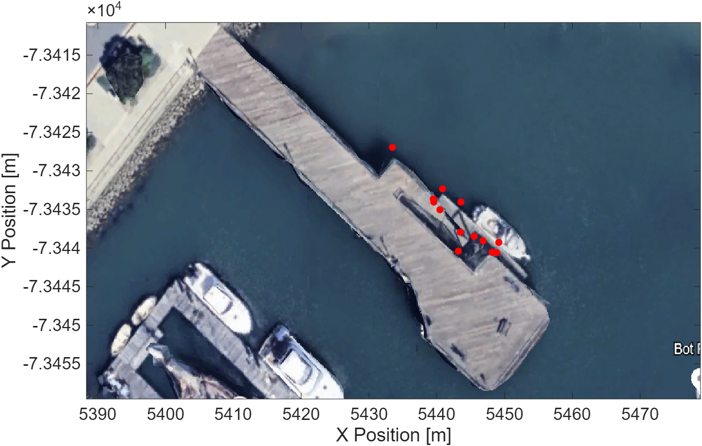
To collect experimental data, the AUV was deployed along the edge of Dana Point Pier in increments of about 1.5m away from each previous trial. This location was chosen for the easy monitoring and retrieval of the AUV, and the ability to deploy the AUV in a gridlike path to collect magnetic flux density readings at approximated locations, without using surface control or the unreliable AUV GPS readings. Figure X shows the deployment locations as red dots on a map of Dana Point Pier. The plotted points may not be accurate because the latitude and longitude of deployment locations and image cropping bounds were approximated on Google Maps.
Data was processed by plotting the collected pressure, temperature, and magnetic flux density readings in each deployment over time as separate plots in MATLAB. Since pressure and temperature values were recorded using an Analog to Digital Converter (ADC), the values were converted to voltages using \(V_{circuit}=0.0032D\), where \(V_{circuit}\) is the output voltage of the circuit in V and D is the unitless digital output recorded by the ADC. Afterwards, they were converted to depth and temperature using the relevant calibration curves. Deployments which resulted in data that did not match expected values were flagged for further analysis. However, the collected data from each sensor was fairly consistent between all deployments.
Deployment Safety
To prevent environmental waste, a tether was tied to the AUV and held onto during deployments so that if the motors failed, it could be brought back to a retrievable location easily. Parts that could easily disconnect from the AUV, such as pool noodles, motors, and ballasting weights, were taped and zip-tied to the frame to prevent them from being lost in the water.
To ensure personal safety, both boxes were checked to be sealed with no protruding wires before deployment to prevent the electronics from getting wet and producing hazardous shorts that deployment personnel could touch. Unexpected occurrences, such as the hardware sparking and foaming, led to immediate deployment abortions, and relevant hardware was replaced before redeployment as needed.
Results and Analysis
Pressure Sensor and Depth Control
During each deployment, the AUV recorded depth continuously while performing P-control. Figure X shows the depth tracked during one deployment. The pressure sensor collected very accurate depth measurements, as the recorded depth fluctuated by at most ±0.032m when the AUV was at the surface or bottom of the ocean. Furthermore, the \(R^2\) value of the calibration curve was 0.996, suggesting the calibration curve equation used can predict depth based on output voltage very accurately.
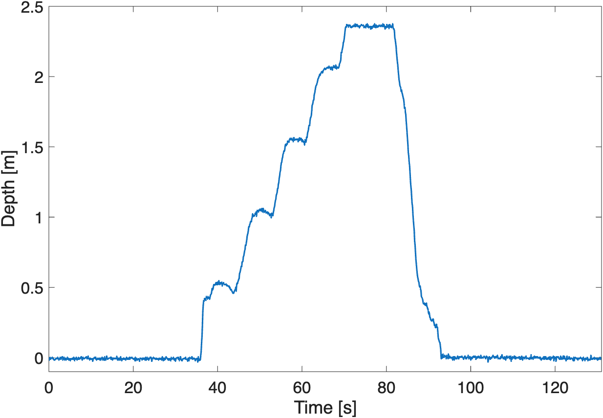
The P-control was successful in holding the AUV’s position at each waypoint, as over the 5 seconds it had to hold its position for, the largest overshoot was by 0.048m when the AUV attempted to reach the first waypoint at 0.5m. After the overshoot, the AUV almost immediately corrected itself and held its value within ±0.02m before moving to the next waypoint. These depth variations are negligible compared to the deepest deployment of 3m in one trial. The depth control algorithm as a whole was also successful, as the AUV was able to determine it had reached the seafloor at around 2.35m below the ocean surface and autonomously came up. The time it took for the AUV to determine it had reached the seafloor varied greatly between trials. In one trial, the AUV ran the depth control algorithm for around 10 minutes before resurfacing. This is because the algorithm determines if the AUV has reached the seafloor when the difference between maximum and minimum output voltages in a range of about 20 seconds is less than 0.05V. Environmental factors, such as other AUVs being simultaneously deployed, could have shifted the AUV underwater in this time frame and changed the output voltage, thus increasing the time spent on the seafloor.
Thermistor
The AUV also collected temperature measurements continuously. As shown in Figure X, the collected temperature readings of a near-constant 28.0545°C were significantly higher than the obtained ground truth measurement of 18.4-18.7°C from probing the seawater at the surface with a digital thermometer. Upon further analysis, these readings indicated that either the op-amps or the Teensy 4.0 likely railed out, because an output voltage of 0V from the thermistor interface circuit would result in this exact temperature value. Even for the non-constant values, such as the two sharp peaks in Figure X, the temperature is significantly higher than the expected value.
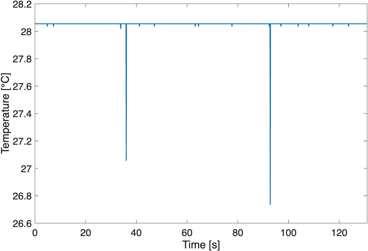
It was first hypothesized that the motors running drew too much current, and this could have prevented the thermistor interface circuit from working properly. However, data from the thermistor was collected in the air and with the motors running, and the thermistor read reasonable values of ~13°C. It was then hypothesized that because the thermistor had reasonable readings in air and only railed out in the water, part of the thermistor was shorting in the water. The ends of the heat-shrunk areas of the thermistor were probable entry points for seawater, so they were dried and then wrapped with Parafilm in an attempt to waterproof them. However, this produced the same issue of railing out. The thermistor was then detached from the AUV, and its wire was slowly dropped deeper into the water. When only the head of the thermistor was in the water, output voltages indicated a temperature of around 12°C, but when more of the wire was put into the water, the circuit railed out. This means there was likely a nick somewhere along the wire insulation, and this caused the thermistor to short and effectively make its resistance negligible in seawater. The exact location of this hypothetical nick could not be determined. The obtained 12°C temperature is still significantly different from the ground truth measurement, indicating a separate issue with the thermistor interface circuit. One possible explanation for this issue is that, since resistors were desoldered and replaced to debug the thermistor interface circuit at Dana Point, the individual resistor values could have changed due to soldering at high temperatures of around 700°F.
Magnetomer
The magnetometer also behaved strangely in the water. As shown in Figure X, when the AUV started descending in the ocean, the magnetic flux density reading would spike to an invalid value (874.733µT is out of the range of the RM3100’s readings) and then read a constant value for the rest of the deployment.
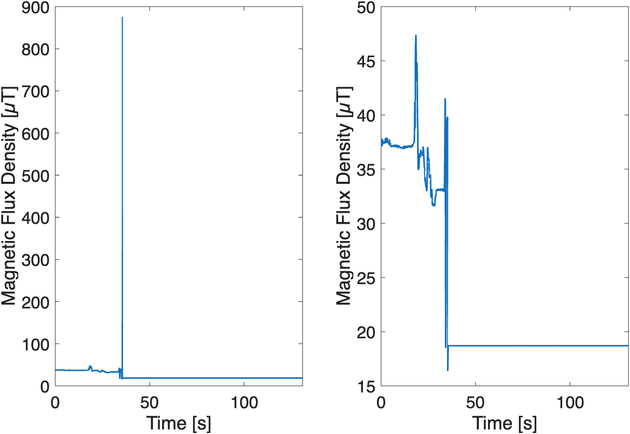
It was hypothesized that the motors produced electromagnetic interference (EMI), which interfered with the I2C data transmission. EMI can produce three types of errors in I2C sensors: no communication, erroneous values, and permanent values from the sensor. This aligns with the collected data, in that the large spike is an erroneous value, and the constant value indicates either no communication or a permanent value being transmitted. To confirm this theory that motors producing EMI interfered with the magnetometer’s I2C communication, a recreation of this spike and flatline pattern was attempted by taping a motor to a waterproof box with the magnetometer and circuitry, running the code used at Dana Point on the same hardware, and dropping this setup in a tank of freshwater. With this setup, the magnetometer produced steady readings without any anomalous peaks or flatlines. The magnetometer was then taken out of the box and pressed directly against the running motor. This produced the peak and flatline pattern. Upon further investigation with an oscilloscope, it was found that the DRDY pin output a constant HIGH signal when pressed against the running motor, meaning new data was never being pushed to the relevant registers. Because this pattern only occurred when the magnetometer and motors were far apart in seawater and not in freshwater, it is hypothesized that the seawater amplified the EMI more than freshwater, causing interference only in the Dana Point deployments.
Conclusions
This project aimed to determine the effectiveness of calculating geostrophic flow through pressure and temperature measurements and mapping seafloor debris through magnetometry.
The pressure sensor was the most successful sensor used. Its calibration curve had an extremely high \(R^{2}\) value of 0.996, meaning its output voltages were well correlated with depth, even after amplification from the circuit. Additionally, it worked well with the depth control algorithm, in that the AUV correctly held itself at each waypoint within ±0.02m, correctly determined it had reached the sea floor with readings fluctuating by only ±0.032m, and surfaced on its own.
The thermistor did not produce any reliable readings underwater. It railed out at around 28°C in each trial. However, from testing, this was likely due to a break along the wire, which would have caused the sensor to short, and this is easily fixable through additional heatshrink or coating the wires with some waterproof material. The narrow 95% confidence intervals for the Steinhart-Hart coefficients from calibrating the thermistor imply that it was well calibrated and had high precision, and fixing this issue would have produced very accurate sensor readings.
The magnetometer did not produce sufficient data to locate seafloor debris at Dana Point. Although it failed to produce reliable readings at Dana Point, readings in the air fell within the expected range. Thus, further development and exploration into its behaviour with EMI from motors in seawater could improve the reliability of this sensor in the ocean, so that it could be used in a similar AUV.
Due to the inadequate temperature and magnetic flux density data, geostrophic flow was not calculated, and a map of seafloor debris was not obtained.
The measured temperature from the thermistor circuit had serious discrepancies with the probed measurement, and the magnetometer readings could not be reasonably correlated with the true magnetic flux density underwater. Future exploration would benefit from finding a better method to waterproof the thermistor and prevent shorts along its path, and exploration into preventing EMI from disrupting I2C sensor readings. After resolving these issues, attempting to characterize geostrophic flow and locating ferromagnetic debris on the seafloor using the collected data would confirm whether utilizing pressure, temperature, and magnetic flux density is a feasible method for accurately locating ocean wreckages.
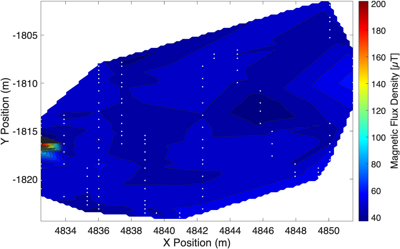
As a proof of concept, Figure X shows a contour plot of magnetic flux density collected by scattering neodymium magnets on the floor outside of Parsons Engineering Building in Claremont, CA, and plotting collected magnetic flux density readings from the magnetometer corresponding to GPS-obtained positions. The peak value at around (4833, -1817) and other elevated values at (4846, -1813) and (4839, -1815) roughly correspond to the magnet locations. Assuming more reasonable magnetic flux density readings can be obtained in the ocean, a similar plot outlining the location of ferromagnetic materials on the seafloor could be acquired.
Besides improving the method outlined in this paper, work using other sensors that would encompass a more comprehensive view of seafloor debris should be considered. Sensors such as high-resolution side-scan sonar could be used to confirm if detected ferromagnetic materials on the seafloor are actually relevant debris or just part of the ocean’s natural ecosystem. In addition, the high error in the GPS made surface control at Dana Point very unreliable and unusable. Using a more accurate GPS module would increase the accuracy of plotted values in the contour plot and enable the AUV to traverse to various surface waypoints and start depth control at remote locations autonomously.
Final Paper
Read through my IEEE-formatted technical report about this project here!